Linear Language Models
Background
In the field of numerical analysis one can generally say that there are a number of differences between linear and nonlinear processes, at least at a very high level. Perhaps most notably, linear transformations may be completed in one effective ‘step’ whereas nonlinear transformations require many ‘steps’. Whether this is accurate or not in practice is somewhat dubious, but for our particular application it will indeed be.
This is relevant because we can get an idea of how to make an extremely fast (to run, that is) language model by considering what exactly happens during autoregressive inference. When one considers autoregressive inference, it is generally noted that models like Transformers that compare all tokens to all other tokens scale with $n^3d$ time complexity without caching, and $n^2d$ with caching for $n$ tokens and hidden dimension $d$. It is less appreciated that inference time also depends on the number of layers of linear transformations in a model $l$, as because typically each layer is separated from each next layer by one or more nonlinear transformation (layer normalization, ReLU, GeLU etc.) such that the actual time complexity becomes $n^2d^2l$ as each of the $n^2$ token comparisons require $l$ steps.
Clearly it would be advantageous to reduce the number of layers in a model, but how can this be done while maintaining an efficiently trainable architecture? To start to answer this question, one can instead ask the following: ignoring trainability, what is the minimum number of layers in a causal language model? The answer is straightforward: a one-layer model contains the fewest layers, and a one-layer model in this case is equivalently a fully linear model. The question then becomes whether or not a linear or nearly-linear model is capable of being trained effectively, either on a small dataset like TinyStories or a larger dataset like the Fineweb.
For small datasets like TinyStories, the answer is somewhat surprisingly yes: fully linear language models are capable of generating gramatically correct text, although is a good deal less efficient to train than a nonlinear model.
Linear Mixer Architecture
Before proceeding further, however, it is best to understand a few theoretical arguments for and against the use of linear models. The arguments for mostly revolve around their utility: they are fast (because they can be mostly or wholly parallelized on hardware), easy to optimize, and somewhat more interpretable than nonlinear ones. The downsides revolve around their lack of representational power.
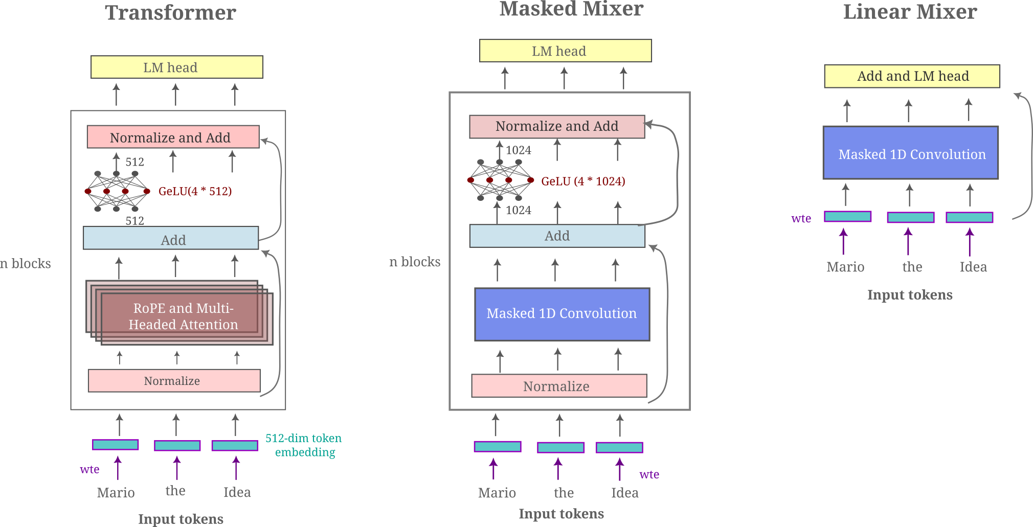
How might one go about converting a masked mixer into a linear model? We will take the approach to remove nonlinear transformations and optimize the resulting linear model to train most efficiently using adaptive versions of stochastic gradient descent. We start with a masked mixer as this model may be thought of as a transformer with self-attention replaced by a single linear transformation (a masked convolution and proceed to linearize the rest of the model.
Besides removing nonlinear activations, we must also deal with layer normalizations, which are defined as follows: for a specific layer input $x$, the output $y$ is
\[y = \frac{x - \mu}{\sqrt{\sigma^2 + \epsilon}} * \gamma + \beta\]where $\gamma$ and $\beta$ are trainable parameters (which are usually held in very high precision) and $\mu, \sigma^2$ denote the mean (expectation) and variance of the random variable $x$. This is clearly a nonlinear operation (although it could be transformed into a linear one) and so we will simply remove this transformation for now.
We also remove superfluous linear transformations: in particular the feedforward module of a transformer usually contains a up projection $U$, nonlinear activation, and down projection $D$. Without the nonlinearity, we are left with a sequence of transformations applied to input $x$ expressed as $DUx$, but we can compose these two linear transformations into one, ie $DUx=Wx$, for efficiency. Furthermore, we can also compose this feedforward weight matrix with the language modeling head layer $H_{lm head}$, as $HWx = Qx$ for all matrices $H, W$ and some $Q$. We could go further and continue to compose layers together, but as we will see in the next section this is surprisingly not always benefical for efficient training.
The linear masked mixer architecture we use may be compared with the transformer and masked mixer diagramatically. In the following depiction, all nonlinear transformations are colored red and all linear transformations are blue or purple.
We can be confident that a linear model will not have the representational power of a nonlinear one from an abundance of arguments for this idea. But can a linear model be trained to effectively model language? At least for simple langauge datasets such as TinyStories (synthetic paragraph-length stories written as if from a five-year-old’s perspective, albeit much less creatively than what you would get from a real five-year-old), the answer is suprisingly yes as we will see below. This dataset is certainly much less challenging to model compared to broad text corpora with code, mathematics, web pages, and books that are commonly fed to frontier models today, but it is important to note that much is included in modeling even TinyStories; factual recall (names and places and simple events), grammar, story coherence and context for a few.
Nearly Linear Models
Before proceeding to fully linear models, it may be beneficial to observe how almost-linear models (with only one nonlinear activation layer) perform when modeling TinyStories. Recalling that single-hidden-layer (with practically any nonlinear activation) neural networks are universal for all computable functions, we would expect models of sufficient size of this architecture to be capable of arbitrarily good TinyStories modeling, but it remains to be seen whether or not these models are practically trainable given limited hardware.
The following figure shows how a model with ReLU activations after the convolution scales: here we use a tokenizer of size 4096 and hidden dimensions as denoted.
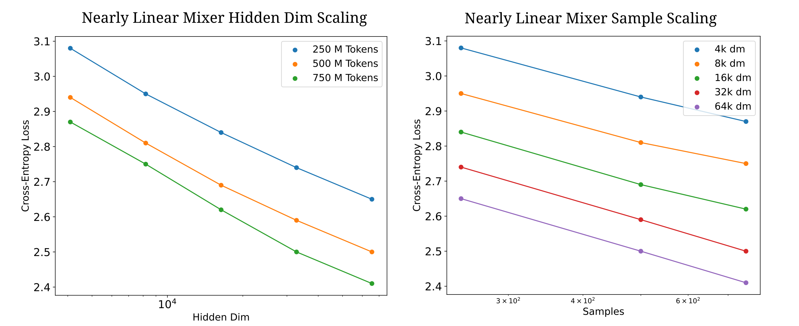
This architecture performs in a superior manner to a linear mixer with inter-token transformations conv1D -> gelu -> conv1d (such that we only have $n_{ctx}$ nonlinear transformations in the model), as for that architecture we have the following cross-entropy losses:
| dm | 4096 | 8192 | 16384 |
|---|---|---|---|
| 1e | 3.25 | 3.27 | 3.24 |
| 2e | 3.09 | 3.04 | 3.00 |
| 3e | 3.02 | 2.94 | 2.87 |
Whereas for a one-layer mixer or transformer (with nonlinearities between intra-token feedforward transformations), we have
| dm | Mixer 4096 | Mixer 8192 | Llama 4096 |
|---|---|---|---|
| 1e | 2.51 | 2.38 | 2.30 |
| 2e | 2.36 | 2.25 | 2.18 |
| 3e | 2.28 | 2.16 | 2.12 |
Linear models inference with O(log n) complexity
What is necessary for efficient TinyStories modeling in terms of model linearity? Some experimentation can convince use that simply stacking linear layers does not increase training efficiency, and indeed decreases it slightly. This is true both when the entire linear mixer architecture contains more than one module, or else when we use two or three or more linear transformations after the convolutional layer.
These results are to be expected from the fundamentals of linear algebra, where multiplication by multiple matrices in succession may always be reduced to multiplication by a single matrix (assuming no nonlinearities are added between layers). This is true regardless of whether or not the weight matrices expand the vector’s width at intermediate stages or not: for example if $W$ is a 8x2 (m by n, rows by columns) matrix and $H$ an 2x8 matrix such that $Wx$ expands $x$ by a factor of four and $H(Wx)$ reduces $Wx$ by a factor of four again then one can always make an equivalent matrix $Q$ that is 2x2.
Therefore one would not expect for matrices with ‘expanded’ hidden layers in a linear model to be beneficial, and this is true for TinyStories modeling when one uses a tokenizer of fixed size. To see why this is, consider the computational graph of an $n_{ctx}=3$ linear mixer. In the following figure, we assume that the tokens have been pre-converted to one-hot vectors and denote vectors in lower-case italic letters, constants in lower-case letters, and matrices in upper-case letters.
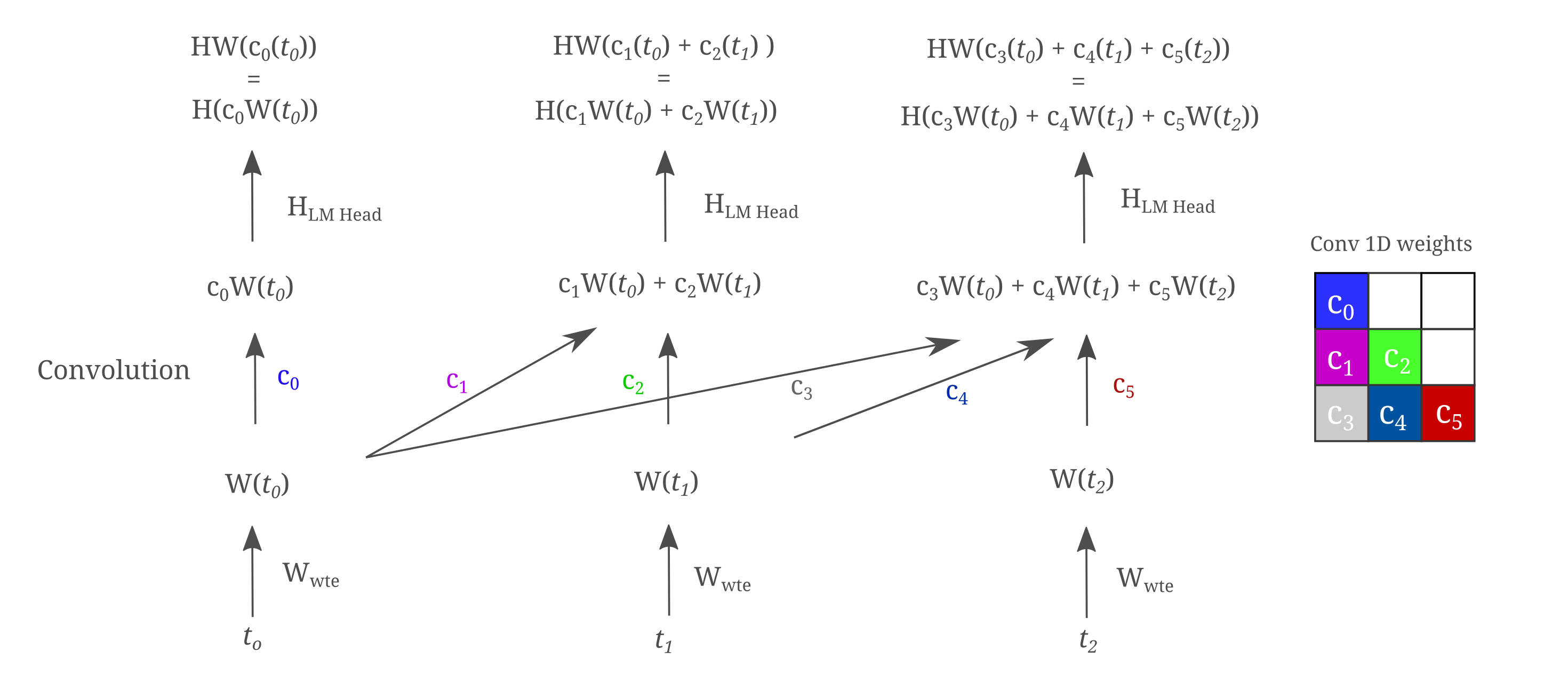
The equivalence in the top row to the second row may be seen as all convolutional weight elements are constants, and scaling a given matrices’ row before multiplying to another matrices’ column (ie forming a dot product) is equivalent to multiplying first and scaling after, and follows from the linearity of matrix multiplication. Now note that $HWx$ fulfills the same matrix multiplication we saw before: one should not expect to have any performance increase if $W$ expands the dimensionality of $x$ and $H$ decreases it, as one can always find a $Q$ that is equivalent that does not expand $x$.
For inference, the linear mixer can be further composed: given trained weight matrices $W$ and $H$, we can multiply these to find $Q$ that will be much smaller if we use a larger dimension than the tokenizer size $d_m > \lvert t\rvert$. Recalling that $t_n$ is a one-hot vector and $c_n$ a constant, computation of $c_n t_n$ is simply a scaled one-hot vector and is extremly fast as well, and furthermore adding these scaled one-hots together is fast and requires only $n$ operations, resulting in a vector $a$ of size $\lvert t \rvert$. All together, the computation of each next token is simply a single matrix-vector multiplication once the vector $a$ has been formed
\[O_n = HW(c_0 t_0 + c_1 t_1 + \cdots + c_n t_n) \\ O_n = Q(a_n)\]Thus no matter what the inner dimension of $H, W$ are (ie the expansion factor, assuming m>n for $W_{m,n}$) the operations performed are equivalent to a linear model with no expansion and $Q$ substituted for $HW$. Experimental results bear this out: regardless of whether one uses m=n or m=4n or m=8n, we see identical training efficiencies when the resulting model is applied to TinyStories. This is notably not the case for $m<n$, as in that case the resulting matrix $Q$ is not full rank and thus the model can learn only a limited subset of all potential matrices representing the composed weights.
Composing these transformations allows for extremely efficient inference via parallelization, as inference with a linear model is simply a linear recurrence. To see why inference is so efficient, observe that for any given token $t_n$ we want to generate, we simply form a polynomial of powers of $Q$ with scaled (one-hot) $t_0$. Here we assume that the output after transformation $H$ is sufficiently close to a one-hot output such that it can be transformed by $W$ without loss in model performance (which is not necessarily a safe assumption).
\[t_1 = HW(c_0 t_0) = Q(c_0 t_0) \\ t_2 = H(c_1Wt_0 + c_2W(HWc_0 t_0)) = Q(c_1 t_0) + Q^2(c_0 t_0) \\ t_3 = Qc_3t_0 + Q^2c_4c_0t_0 + Q^2c_1c_5t_0 + Q^3c_0t_0\]This allows one to calculate $t_n$ and $t_{n+1}$ in parallel, and indeed one can calculate all next tokens in parallel because of the linearity of the model in question. To further save computational costs, for $N$ tokens one wants to generate one can compute the $N$ powers of $Q$ in $O(N \log m)$ time and then save the single column of each matrix that is required to compute the multiplication with $t_0$, which requires $m \times N$ memory. If this is done, each polynomial term reduces to a single scaling of a vector and the computation of the polynomial as a whole is reducible to vector addition, which may be achieved in $O(\log N)$ time via prefix sum. In this sense, one can cache vectors and compute all next tokens required in parallel via cache lookups and addition with $O(log N)$ time complexity (and $O(N)$ space) without any modifications to the mixer architecture itself.
Linear Mixer Scaling
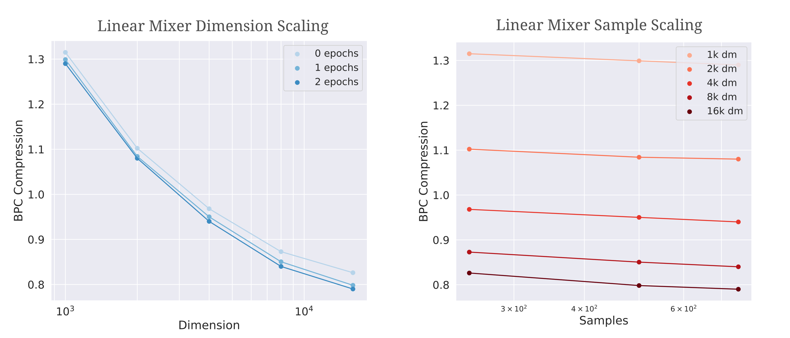
How can one increase the dimensionality of a linear mixer model? As we are effectively limited to $W_{m, n}, m=n$ where $m = \vert t \vert$ we can simply increase the tokenizer size to increase the dimensionality of the transformation $W$. But this presents a problem: one cannot directly compare cross-entropy loss values of models with different tokenizers, as the amount of information necessary to match a target distribution clearly changes depending on how many elements exist in that distribution (as guessing one of two values is easier than guessing one of a thousand). We must instead convert our cross-entropy loss values to a more universal measurement, which we choose somewhat arbitrarily to be compression in terms of Bits per Byte (of text). The cross-entropy loss on this page is equivalent to negative log likelihood loss $\Bbb L$ on softmax-transformed logits, which happily makes calculation of bits per byte straightforward.
To find the number of bits per byte compression each model achieves, first we calculate the average number of characters per token $L_t / L_c$ and then find the model’s loss and calculate as follows:
\[BPC = (L_t/L_c) * \Bbb L / \ln(2)\]Now able to compare compression results between models with different tokenizers, we find that compression does increase as $d_m=\vert t \vert$ increases, but that there is rather fast saturation with respect to compression per sample trained upon relative to the nearly-linear models above.
The increased compression (modeling ability) resulting from larger linear models suggests that a sufficiently large linear model would be capable of accurate language modeling. How can this be, given the well-known limitations of linear models? The answer is that dimensionality can overcome nearly all barriers, and to see why we turn to a classical challenge brought to fully linear models.
When perceptrons were first introduced by Rosenblatt and colleagues, a criticism levelled at them by arguably the (at the time) most well known AI researcher (Minsky) was aas follows: these models may be capable of much but cannot be that good, as they cannot compute a function as simple as XOR. The reasoning is as follows: linear perceptrons define functions that linearly separate space, ie slice the input into parts along lines. A brief glance at XOR in two dimensions (variables) shows that clearly no line can separate the true from false points, and this criticism was successful enough to hinder research into perceptrons for some time.
WIth more discernment, however, it is clear that this particular argument is somewhat specious: a linear function actually can indeed separate XOR points and the key to this is to observe what happens when we embed the two-dimensional XOR into three or more dimensinos: if there is a nonzero distance between either false or true points, a linear segmentation sucessfully separates the two pairs.
More generally, as the dimension of the embedding space increases it becomes less and less likely that any specific configuration of points cannot be linearly separated with some mild assumptions on the nature of those points. This phenomenon is essentially the mirror image to what statisticians refer to tas the ‘curse of dimensionality’, where accurate interpolation becomes difficult when the dimensionality of the data becomes large: if the number of embedding dimensions exceeds the number of data points, there will be a way to linearly divide any two or more sets of points unless they exist completely inside a smaller subspace.