Language Mixers III: Optimization
Training large models takes a large amount of compute, but why this is the case is not immediately apparent as it does not necessarily follow from the model size alone. On this page we take a first-principles approach to understanding why this is the case through the lens of numerical optimization. We will explore the use of optimization methods that are theoretically much faster than gradient descent in the context of linear transformation optimization.
Background
The process of training the deep learning models that are used for language and vision modeling may be thought of as a specialized type of unconstrained nonlinear optimization, one in which the function or model being optimized is itself composed of many linear transformations separated by various normalizations and nonlinear functions, where each linear transformation and linear part of the normalization (but typically none of the nonlinear functions).
If one were to take a number of mid-20th-century numerical analysts and show them the optimization procedures used today for large deep learning models, I think it would be safe to say that they would be fairly suprised at the use of methods that give virtually no guarantees of convergence, and that converge slowly when they do at all with respect to asymptotic order characteristics. This is because there have long been known to exists methods by which linear transformations may be solved explicitly, or for that matter methods that minimize nonlinear transformations with much faster convergence characteristics, that are completely absent from today’s optimization methods.
This work will focus on the use of two methods for optimization that are in theory much faster than gradient descent, and detail why they are difficult to apply to even relatively simple language models. We then explore what exactly is necessary for convergence of large language models in the context of gradient descent-based optimization.
Introduction: Classical optimization methods that converge quickly
For most machine learning tasks, we are given a system of equations (a ‘model’) and want to maximize the performance of this model on some given task, which is usually framed as minimizing a loss function on that task. If one is given a list of equations and asked to provide values that minimize the output of this equation, the approach one would want to take depends considerably on what type of equations are given.
If the equations are linear and the loss function is a quadratic function like mean squared error, we can use some principles from calculus to solve the equation in one mathematical operation. It should be noted that this one operation will almost always require many computational iterations to complete, so it should not strictly speaking be thought of as only one step in a machine. Nevertheless, this can be viewed as perhaps the fastest optimization method possible.
If the equations are nonlinear, or the loss function is more complicated than a quadratic (and in particular if it is non-convex) then we must turn to other optimization methods that are typically iterative in nature. The methods commonly used for deep learning model optimization are based on gradient descent, in which many small steps are taken each in the direction of steepest decline in the loss function. If gradient descent-based optimization converges (meaning that it reaches a sufficiently small loss value) then the convergence occurs linearly: as we take a step of no more than the learning rate size for each iteration, we need at least $n$ steps for our initial model to reach the point of convergence. More precisely,
\[|| x_{(k+1)} - x^* || = O(|| x_{(k)} - x^* ||) \tag{1} \label{eq1}\]This is somewhat of an oversimplification of today’s methods, the most common of which being AdamW which typically one uses adaptive learning rates to estimate the momentum of a point in its loss trajectory, such that the accuracy of applying \eqref{eq1} may be questioned. However, it can be shown that AdamW and other moment-estimating methods cannot converge any more quickly than pure gradient descent with well-chosen parameters (ref) such that \eqref{eq1} is valid.
Happily there are other methods that converge much more quickly: one in particular is Newton’s method. This name is somewhat confusing because it is applied to two different related optimization techniques, one that is commonly applied to minimizing a loss function for nonlinear models and requires the computation of Hessian matrices (which is usually computationally infeasible for large models) and one that finds the roots of a function and requires only the Jacobian of the weight matrix, which in the case of functions $F: \Bbb R^m \to \Bbb R^1$ is equivalent to the gradient. This method is iterative but takes large steps, solving a linear equation for an intercept at each step. Newton’s method converges quadratically provided some mild assumtions are made as to the continuity and nonsingularity of the system of equations,
\[|| x_{(k+1)} - x^* || = O(|| x_{(k)} - x^* ||^2) \tag{2} \label{eq2}\]This may not seem like much of an improvement on gradient descent, but it is actually an enormous improvement in terms of asymptotic characteristics. Say you were given some target $x^*$ that required $n$ steps of gradient descent to reach from an initial value $x_0$. The same target would be expected to require only $\sqrt{n}$ steps for Newton’s method, which is a substantial improvement as $n$ increases.
Ordinary Least Squares via the Normal Equation
Suppose we were told that a linear model would be perfectly acceptable for language tasks and that we can choose to minimize any loss function we wanted. In this case perhaps the simplest conceptual approach is to choose a quadratic loss function like mean squared error and simply solve the resulting equation for the model parameters $\hat \beta$ given input $X$ and target output $y$, and for now we can avoid the details of exactly how this would be implemented. In the case of a $\beta$ being a square weight matrix of full rank, we can simply solve the model equation to get our desired weights (with zero loss):
\[y = X\beta \implies X^{-1}y = \beta\]This is usually not possible as a weight matrix is in general non strictly invertible, such that there could be many or more commonly no exact solutions to the equation. In this case we have to decide on a loss function and find some value for our weights that minimizes this loss. In the common case in which there are no exact solutions for the equation, we can still solve for a desired weight value if the loss function is sufficiently simple. Mean squared error is happily simple enough to solve when applied to a linear regression, and there are a number of ways to approach this problem.
One of the most straighforward ways of deriving this equation is to simply solve the system of equations present when we set the gradient to be zero,
\[\Bbb L = || X \beta - y||_2^2\]which can be done via distribution and gradient application
\[\nabla_\beta (1/m) (X\beta - y)^2 = 0 \implies \\ \nabla_\beta (\beta^TX^TX \beta - \beta^TX^Ty - y^TX\beta - y^Ty) = \\ 2X^TX\beta - X^Ty - y^TX = 0\]Recalling that $y$ is a vector, we have $X^Ty = y^TX$ as both are the vector formed by the dot prods of columns of $X$ with y, so we have
\[2X^TX\beta - 2X^Ty = 0 \implies \beta = (X^TX)^{-1}X^Ty\]This is unfortunately not the most numerically stable equation for larger matricies $X$: we can implement this equation directly using a tensor library like Pytorch as follows, and upon doing so we will not find that the parameters we obtain do not minimize our MSE loss function even for relatively small equations.
beta_hat = (torch.inverse(X.T @ X) @ X.T) @ y
Happily, however, there is a more stable formulation utilizing the singular value decomposition components $U, D, V$,
\[\theta_W = \lim_{\alpha \to 0^+} (X^TX + \alpha I)^{-1}X^T y \\ = X^+y = VD^+U^Ty\]where $X^+$ denotes the Roy-Moore Pseudo-inverse of $X$. This can be implemented simply in torch as follows:
beta_hat = torch.pinverse(X) @ target
We will use a small linear language model to test the ability of the normal equation to minimize loss as this model has only three linear transformations: a token embedding layer, a masked convolution, and a language modeling head layer. In principle, however, a model of any type could be used, as long as the last layer is linear and we optimize the weights of that layer. This is because we can decompose the model output to be the input to the lm_head transformation (which is linear) multiplied by the weights of that transformation, which in traditional notation is
The wrinke is that we need to convert integer tokens to vector spaces to be able to measure mean squared error. We can do this using the one-hot pytorch transform as follows:
target = torch.nn.functional.one_hot(train_batch, num_classes=len(tokenizer)).to(torch.double).squeeze(1) # [b t e] shape
Mean squared error is not a perticularly good choice of loss function for categorical data such as token identity, but we can make it a somewhat more reliable loss function by scaling our one-hot to be approximately the size of the tokenizer: for example, given a tokenizer with the size of a few thousand tokens we can scale the one-hot from one to one thousand. This is helpful because it increases the penalty of any optimizer choosing a function that assigns all inputs to the origin: in this case, the trivial reduced mean squared error is $1000^2/4096 \approx 244$ instead of $1^2/4096 \approx 0.001$.
For causal language modeling we want to compare the model’s output at position $n$ to the token at position $n+1$, so in this case we want the input to be the activations of the last hidden layer (which is the input to the lm_head layer in our model) shifted so that we mask the last token, and the target shifted to mask the first token.
output, X = model(train_batch) # X is the input to the lm_head, ie tensor of activations
X = X[:, :-1, :].contiguous()
target = target[:, 1:, :].contiguous()
We can apply the normal equations to this model by saving the activations of the input of this lm_head layer, converting the target output to one-hot tensors for use with mean squared error loss, shifting the target and inputs for causal language modeling (next token prediction), computation of the minimal lm_head weight, and assignment of that weight.
Finally, we don’t need to compute gradients when using the normal equations for loss minimization so we can wrap our function using the handy @torch.no_grad() to save memory. All together, we have
@torch.no_grad()
def normal_solve(model, train_data, scale=1000):
    train_batch = train_data.unsqueeze(0).to('cuda')
    loss, output, X = model(train_batch, labels=train_batch)
    target = torch.nn.functional.one_hot(train_batch, num_classes=len(tokenizer)).to(torch.float).squeeze(1) * scale # [b t e] shape
    X = X[:, :-1, :].contiguous()
    target = target[:, 1:, :].contiguous()
    prefix = torch.pinverse(X)
    beta_hat = (prefix @ target)[0] # automatically forms the batch dim, squeezes this here
    model.lm_head.weight = torch.nn.Parameter(beta_hat.T)
    loss, output, X = model(train_batch, labels=train_batch)
    return loss.item()
When we observe the pre-optimized loss, we find almost exactly what we were expecting: for $d_m=128$ model with a tokenizer of size 4096 and a context window (meaning the number of tokens in the sequence we are modeling), we have
Starting loss: 244.5254053321467
Ending loss: 0.9978399276733398
This ending loss may be considered the irredicuble error that is associated with imprecise numerical computation: with 128 equations and 128 unknowns, we should be able to find a weight configuration that gives us an ending loss of 0.
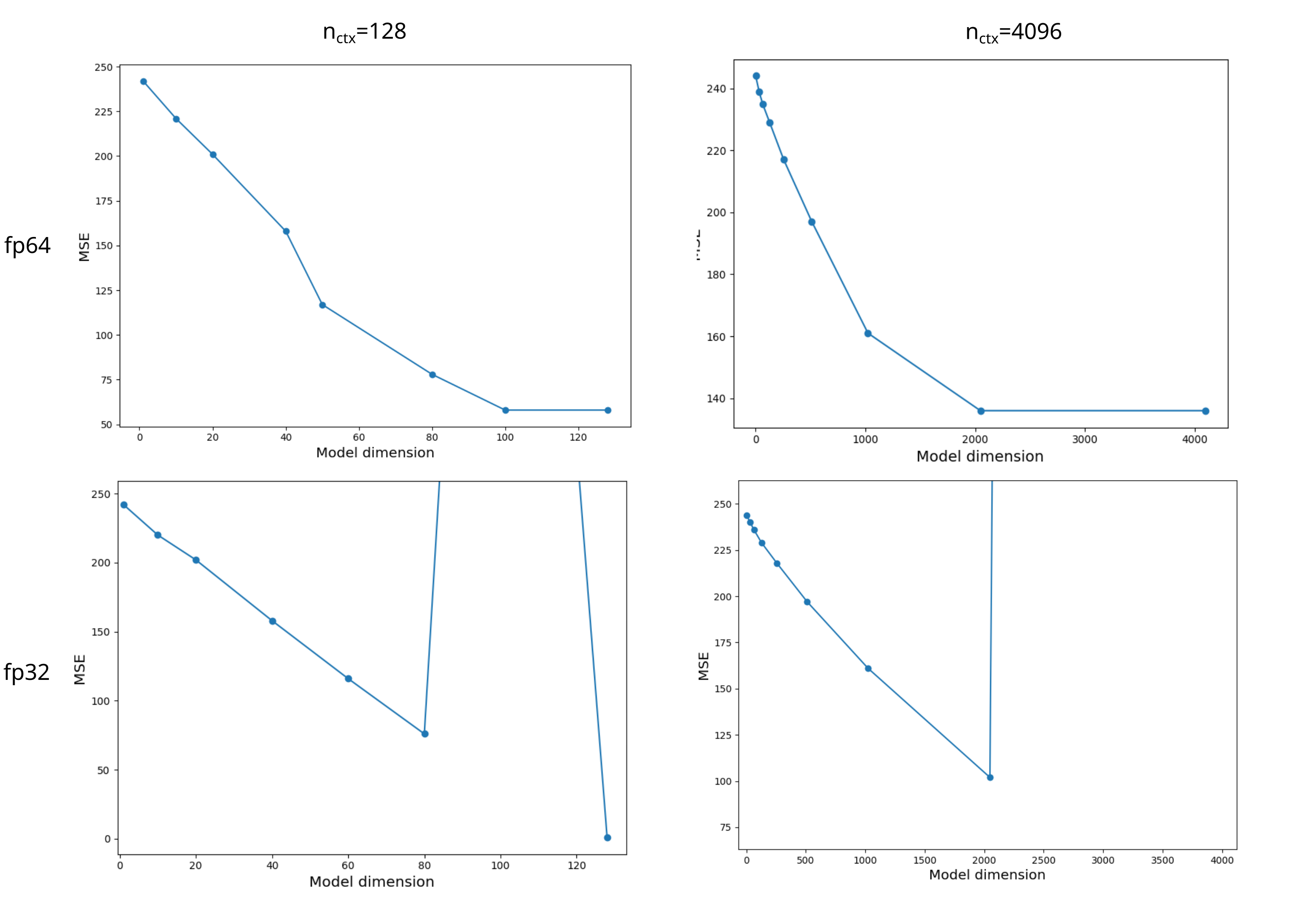
Floating-point instabilities whilst solving the normal equations
Interestingly, the ending loss is usually much higher than what was found above: repeating the same calculations in fp32 rather than fp16 takes a good deal longer and yields
Starting loss: 244.5254053321467
Ending loss: 58.21005218079172
When we plot the mean squared error loss for
Newton’s method
As mentioned in the last section, there are two related versions of Newton’s method that may be applied to the problem of minimizing an model’s loss function given some data. It is helpful to first understand the differences between these methods and show how they are related before examining how they can be applied to deep learning models. At its heart, Newton’s method is an iterative method that computes the roots (zeros) of an arbitrary equation $f(x)$: given an initial point $x_0$, we perform some number of iterations such that for each iteration at point $x_n$ we compute the next point $x_{n+1} via \eqref{eq3).
\[x_{n+1} = x_n - \frac{f(x_n)}{f'(x_n)} \tag{3} \label{eq3}\]The derivation of this formula is straightforward: given $f$ differentiable at point $x_n$ by definition $f’(x_n) = \delta y / \delta x$. We solve for the $\delta x$ such that $y=0$, meaning that $y=f(x_n)$ and
\[\frac{f(x_n)}{\delta x} = f'(x_n) \implies \Delta x = \frac{f(x_n}{f'(x_n)}\]and add this value’s inverse (additive inverse) to our original point $x_n$ to obtain the next point.
\[x_{n+1} = x_n - \Delta x = x_n - \frac{f(x_n)}{f'(x_n)}\]In the case where our input $x$ is a vector rather than a scalar and our function $f: \Bbb R^n \to \Bbb R^m$ is of many variables, we must compute the Jacobian $J$ of $f$, which is defined as
\[J_{ij}(x) = \frac{\delta f_i}{ \delta x_j}x\]making Newton’s method as follows:
\[x_{n+1} = x_n - \frac{f(x_n)}{J(x_n)}\]For \eqref{eq3} to actually find a root after many iterations, we need a few conditions to be satisfied (Lipschitz continuity and nonsingularity of $f’$ at $x_n$ for example) but most importantly there must actually be a root to find or each iteration will send us off in an entirely incorrect direction. This can be ensured in two ways: one is use an offset such that the zero of the loss is more or less guaranteed to be attainable, and another is to use complex-valued arithmetic.
Using an offset brings a difficulty: what value will give us guaranteed roots? If we use Mean Squared Error loss, we can find minimal loss values for specific input and model combinations using the normal equation method presented in the last section, and simply set the offset to be equal to this minimal loss. In the following function, this offset is set by the loss_constant kwarg.
def newton(model, train_batch, loss_constant=0.01):
    train_batch = torch.stack(train_data[0:1], dim=0).to('cuda')
    for i in range(5):
            model.zero_grad()
            loss, output, _ = model(train_batch, labels=train_batch)
            loss -= loss_constant # subtract suspected irreducible loss so root exists
            loss.backward()
            loss_term = torch.pinverse(model.lm_head.weight.grad) * loss
            model.lm_head.weight = torch.nn.Parameter(model.lm_head.weight - loss_term.T)
    return
Unforunately, application of Newton’s method (even for relatively large loss_constant values) results in explosion of loss rather than minimization when applied to a language task. This can be shown to be a problem of numerical stability, specifically in the dimensionality of the output that we reduce during loss computation (as we will see later). To work around this problem, we can exploit the additive property of gradients, which can be stated as follows: the gradient of the sum of elements is the sum of the gradients. To be precise,
Now what we usually get when we call MSELoss() (or most any other loss function in the Pytorch library) is a scalar output that is the sum or average of each loss component in the output, because one usually wants to use the loss to perform gradient descent and gradients are only defined with respect to scalars. Effectively we as Pytorch to find the gradient of the sum of the loss. To use our additive property workaround, we can specify self.mse = nn.MSELoss(reduction=None) in order to prevent loss reduction and then backpropegate from each element of the loss separately, adding loss gradients to the model weight tensor iteratively. We can then backpropegate from each loss term (retaining the computational graph each time, as Pytorch does not save the graph by default to reduce memory load) as follows:
def newton_components(model, train_data, loss_constant=0.1):
    train_batch = torch.stack(train_data[0:100], dim=0).to('cuda')
    for i in range(10):
        loss, output, _ = model(train_batch, labels=train_batch)
        loss -= loss_constant # subtract suspected irreducible loss so root exists
        loss_terms = []
        for j in range(tokenized_length-1):
            for k in range(len(train_batch)):
                loss[k][j].backward(retain_graph=True)
                loss_term = torch.pinverse(model.lm_head.weight.grad) * loss[k][j]
                loss_terms.append(loss_term)
                model.zero_grad()
        for loss_term in loss_terms:
            model.lm_head.weight = torch.nn.Parameter(model.lm_head.weight - loss_term.T)
    return
Component decomposition-based Newton’s Method is more stable but still results in loss explosion for the large lm_head matrices necessary for typical language modeling tasks. This can be illustrated by restricting the loss we minimize to just a few elements rather than the hundreds or thousands usually used for sequence modeling. For TinyStories inputs where we have a known minimal loss value (found via the normal equations) such that we are guaranteed convergence if the numerical calculations are stable, the component-wise Newton’s method implementation is numerically stable for over a hundred output elements (10 tokens for 10 hidden units each) whereas the standard Newton’s method implementation is only stable for up to around four (2x2), and becomes unstable when we attempt to minimize the loss of only six elements.
We can make this algorithm even more stable at the expense of greatly increased computation by recomputing the gradient after each model parameter update from the components of each loss element.
def newton_components_recalculated(model, train_data, steps=10, loss_constant=0.9):
    train_batch = torch.stack(train_data[0:100], dim=0).to('cuda')
    for i in range(steps):
        for j in range(tokenized_length-1):
            for k in range(len(train_batch)):
                loss, output, _ = model(train_batch, labels=train_batch)
                loss -= loss_constant # subtract suspected irreducible loss so root exists
                loss[k][j].backward()
                loss_term = torch.pinverse(model.lm_head.weight.grad) * loss[k][j]
                with torch.no_grad():
                    model.lm_head.weight-= loss_term.T
                model.zero_grad()
    return
It should be noted that this the above is no longer equivalent to computing and applying the exact gradient: as the model is updated and the gradient re-calculated component-wise, one cannot expect for this form of Newton’s method to be equivalent to the others even with unlimited arithmetic precision.