Masked Recurrent Mixers

The most efficient non-trivial language model for autoregressive inference are models that read the current token, load a fixed memory representing previous tokens, and predict a next token. This is essentially how recurrent neural networks perform inference, such that any model that may be inferenced using this property may be thought of as a kind of RNN. In the past, it was observed that training RNNs requires a reformulation of the inference process to make use of parallelization (or each forward pass may only train using the output of a single next token, rather than all next tokens in a sequence), and that this training is beset by a number of problems once this is done (numerical stability from back-propegation through time, vanishing gradients, slow convergence etc.) such that current large language model architectures that load a variable amount of memory (for example transformers) have provem much more powerful for most tasks, despite their lower inference efficiencies. If we think about this in terms of inference computational efficiency versus training efficiency and task accuracy, it seems that defining a model first by its inference characteristics and then attempting to increase its training and task performance has proven difficult.

On this page we explore an inversion of this approach: we instead take architectures that we know are relatively efficient to train and capable of many useful language tasks and attempt to constrain them to be efficient to inference, while reducing their training and task performance as little as possible. This approach has been followed with varying degrees of success (in particular see Linear Transformers, linear state space models, and Mamba), but the hypothesis is that the masked mixer provides a better starting architecture with which to enforce constraints than the existing alternatives. It is helpful to first consider why this would be, and we do so in the next section, before proceeding to how this may be done and observing the results of doing so.

On this page we refer to linear time and constant space complexity (at inference) as ‘linear’ complexity models.

Background

The first hypothesis is as follows: adapting linear layers in mixers for linear time and constant space complexity sequence modeling should be easier than similar adaptations for self-attention or state space transformations. There are a few reasons why this is expected to be the case: firstly because masked mixers have been found to be efficiently trainable with only a single linear transformation (ie matrix multiplication) between tokens and constraining this transformation to use only $n$ rather than $n^2$ unique values as a Toeplitz matrix does not substantially affect training efficiency, secondly because these inter-token transformations are explicitly rather than implicitly defined on the input dataset, and finally because mixers generally exhibit superior information retention to models of similar computational complexity (transformers for quadratic and Toeplitz mixers compared to Hyena for O(n log n) complexity models).

How do we measure the success of a linear complexity model? The most common way to do so in the literature has been to simply observe the causal training efficiencies of these models (usually in terms of loss per step) compared to those for quadratic-complexity models of a similar parameter number, which stems from the difficulties long observed in training linear-complexity models efficiency. As this is undoubtedly an important metric, we observe this too but modify the definition of efficiency to be compute- and memory-constant rather than parameter-constant, as the latter can give quite inaccurate representations of how efficient a model actually is to train on real hardware. As an example of why this could be the case, consider two models with the same number of parameters but where one model generates double the activations as the other: as batch size and input length increases, the second model will exhibit half the throughput as the first for a constant compute and thus cannot be considered equivalent in real terms.

Of all the other metrics one could observe for linear complexity models, perhaps the most important is the ability of these models to retain and access arbitrary input information. This is because linear-complexity models, unlike quadratic-complexity models, cannot simply ‘look up’ any given input element during the next element prediction because these models store only a fixed representation of the input and are not explosed to the entire input. We draw a distinction between the information present in the input tokens and the information present in the (trained) model’s parameters themselves: an example of text completion that requires the latter would be the answer to the question ‘How many planets orbit around the Sun?’ which is clearly not answerable from the input tokens alone but requires external information, hopefully gained during training.

It is worthwhile to note that causal training efficiencies do not necessarily reflect information access abilities: for a given text sequence, predicting the next word may or may not require the knowledge of many previous words in that sequence. On the other hand, many difficult language tasks that models are commonly applied to today do require near-arbitrary lookup ability: for example, consider code generation in which a model is required to generate a SQL query from a given schema. Although each next token will usually not depend on most of the previous tokens, it may depend on any of the previous tokens and for a long query all the tokens generated together may depend on most of the previous tokens.

The fundamental challenge arbitrary information access presents for linear-complexity models is that without prior information, it is impossible to know ahead of time (ie while processing the input) which tokens will be important in the future and which tokens will not. Models can be trained to guess which tokens will and will not become important, and indeed approach was taken into account when configuring the Mamba architecture. In some respects, however, such guesses are unsatisfactory because they are inherently error-prone due to the inherent degrees of freedom in language. Happily there is an alternative approach: one can instead hope that the linear model’s input representation accurately captures nearly all of the input information, or equivalently that the fixed memory is a near-lossless compression of the input.

These approaches differ in how information addition to memory is considered: the former attempts to add only important information from each token into the fixed memory and the latter attempts to add all information and maximize compression. The motivation for these approaches reflects their ideal outcomes: selective addition is motivated by application to extremely long sequences where it is practically impossible to compress the input with high fidelity, whereas the high compression can only be achieved for a certain size of sequence length assuming the input is relatively information-rich. We note that for high-information inputs such as language, it is practically hopeless to expect any linear-complexity model to be capable of good information lookup if the input sequence increases in length far beyond the compression limit.

Linear complexity models are usually developed from the perspective of feasibility of modeling very long sequences. From the relative compressions achieved by large causal models, it is clear that language is relatively information-rich compared to other modalities common for modelig (images of the natural world, DNA sequences etc). This presents a severe challenge for linear-complexity, constant cache models: inferencing these models on sequences of indeterminate but not excessive length is sure to result in the cache becoming incapable of capturing all input information.

In practical terms this means that we can expect for linear-complexity models to perform very poorly once they exceed a certain number of tokens, the exact number depending on the sequence. We can therefore expect for constant-cache models to exhibit a catch-22 with respect to sequence length: the longer the input sequence, the more computationally efficient they are compared to quadratic-complexity transformers, but the worse they will perform on any task requiring arbitrary information access.

But it is not only length-related computational complexity where linear-complexity models shine: these models also require far less cache memory due to their constant (and for the models on this page, very small) memory use. Specifically, when generating a single sample via autoregressive inference a linear-complexity model requires $O(1)$ space to store model weights, $O(1)$ space for the hidden value cache and $O(1)$ space to store activations, which contrasts to the $O(1)$ space for model weights, $O(n)$ space for hidden value cache and $O(n^2)$ space for activations in the transformer. For the models on this page, the constant factors for this $O(1)$ complexity are very small: most caches are of equivalent space as a single token’s hidden activations, although ocassionally this is increased by a small constant value.

There are two advantages to this low memory complexity at inference. For single sample generation one can attempt to store this cache in fast (shared for L2) on-chip memory instead of global GPU memory for far faster autoregression, although even without such memory management the much smaller memory access required by linear complexity models means that they are much faster to inference due to the fact that most single-sample inferences are limited by global memory bandwith rather than FLOPs. A small cache is also useful for parallelizable sampling: for cached autoregressive generation of $k$ samples each of length $n$ and a per-token constant $c$, a transformer requires a total global memory access of size $k(n^2/2)c$ whereas a linear-complexity model requires a total access of only size $k(n/2)c$.

These considerations provide motivation to aim at a different goal than previous linear-complexity approaches: instead of attempting to design an architecture capable of very long sequence modeling, we instead design an architecture that has a fixed context window for which we know the model should perform well from theoretical considerations with parallelized throughput in mind, and optimize this model for training efficiency and information retention characteristics. We then design efficient inference algorithms for this architecture, and show how this approach can be much more computationally efficient than the transformers of today.

Adapting a Masked Mixer for Linear Time and Constant Space Complexity

We start by briefly describing the architecture of the masked mixer. In short, this is an MLP Mixer (a transformer-like model where attention is swapped for linear transformations) modified for causal language modeling by adding triangular masks to token mixing transformations. These token mixing operations are what has been called ‘data-independent’: for any given input, the weights of these operations are unchanged and only activations change. In constrast a transformer’s attention is a ‘data-dependent’ transformation, as the token mixing ‘weights’ in attention are themselves dependent upon the input data. Much ado has been made about the difference between data-dependent and data-independent transformations, mostly around the fact that data-dependent transformations actually encode families of functions rather than individual functions and thus may explore a larger function space than the alternative. That argument is not convincing to this author both because the space explorable by data-independent deep nonlinear models is itself extremely large (actually complete for all computable functions), because the training process ends with a highly data-dependent model, and because emperical results suggest very little difference in training efficiency or ability between models of these two classes.

Data-independency provides a very nice feature that we will use here for linear-complexity adaptation: we know what each transformation will be and indeed what the matrix values of each vector-matrix multiplication will be ahead of time, such that we can enforce the limitations we want directly to the transformation itself. Suppose we had a model that had a context window of size $n=3$ and in this case, our inter-token mixing operations for a non-headed model $Y = XM$ may be represented as follows: given the input $X$ of all embeddings for each token, we can express the token mixing operation as matrix multiplication of this input by $M$ as being

\[Y = \begin{pmatrix} X_{0, 0} & X_{0, 1} & X_{0, 2} \\ X_{1, 0} & X_{1, 1} & X_{1, 2} \\ X_{2, 0} & X_{2, 1} & X_{2, 2} \end{pmatrix} \begin{pmatrix} a & b & c \\ d & e & f \\ h & j & k \end{pmatrix} + \begin{pmatrix} \beta_0 & \beta_1 & \beta_2 \\ \beta_3 & \beta_4 & \beta_5 \\ \beta_6 & \beta_7 & \beta_8 \end{pmatrix}\]

where $X_{0, 0}, X_{1, 0}, X_{2, 0}$ correspond to the zeroth, first, and second hidden layer activations of the 0th token. For causal models, the weight matrix is masked so that we multiply $X \in \Bbb R^{d \times n}$ by mixer parameters $M \in \Bbb R^{n \times n}$ as follows:

\[Y = \begin{pmatrix} \vert & \vert & \vert \\ X_0 & X_1 & X_2 \\ \vert & \vert & \vert \end{pmatrix} \begin{pmatrix} a & b & c \\ 0 & e & f \\ 0 & 0 & k \end{pmatrix} + \beta\]

In general there is no way to accelerate this matrix multiplication beyond $\mathcal O(n^2.3…)$, and most algorithms for achieving smaller complexity than $\mathcal O(n^3)$ are galactic (impractical on any real hardware. A simple way one can ensure lower complexity is to restrict the structure of the weight matrix $M$ such that certain values appear in certain positions. Perhaps the most straightforward way to enforce a linear-complexity mixing operation is to simply repeat one value per row of $M$.

\[\begin{pmatrix} \vert & \vert & \vert \\ Y_0 & Y_1 & Y_2 \\ \vert & \vert & \vert \end{pmatrix} = \begin{pmatrix} \vert & \vert & \vert \\ X_0 & X_1 & X_2 \\ \vert & \vert & \vert \end{pmatrix} \begin{pmatrix} a & a & a \\ 0 & b & b \\ 0 & 0 & c \end{pmatrix} + \begin{pmatrix} \vert & \vert & \vert \\ \beta_0 & \beta_1 & \beta_2 \\ \vert & \vert & \vert \end{pmatrix}\]

It is worth expanding the equations to convince ourselves that this is indeed a linear time and constant space complexity operation at inference, or equivalently a recurrent operation with constant memory. When we multiply and add, we have the following:

\[Y_0 = a X_0 + \beta_0 \\ Y_1 = b X_1 + a X_0 + \beta_1 \\ Y_2 = c X_2 + b X_1 + a X_0 + \beta_2 \\ ... \\ Y_n = \alpha_n X_n + \beta_m + \sum_{m=0}^{m=n-1} \alpha_m X_m\]

This shows us that we indeed have a linear-complexity operation: at inference for token $n$, we simply load the single value of $\sum_{m=0}^{m=n-1} \alpha_m X_m$ from memory, add the value of $ \alpha_n X_n$, and save the resulting vector $\sum_{m=0}^{m=n} \alpha_m X_m$ to memory. For token $n+1$, we load that sum and repeat.

When we train this model, we see that there is a significant gap in loss achieved per compute applied relative to the unrestricted ($\mathcal O(n^2)$ complexity) masked mixer: for models of size $n_{ctx}=512, n_l=16, d_m=512$, a repeat mixer achieves a cross-entropy loss of 3.465 at 200k steps, whereas the non-headed masked mixer we see a loss of 2.934. There is a substantial improvement in loss achieved at 200k steps (with minimal training throughput decrease if we use four repeat mixer heads instead of one, in which case loss achieved is 3.311 (a four-headed masked mixer achieves 2.889 loss). Dense transformer architectures typically slightly (<5%) outperform masked mixer models given the same compute, so we would expect for the loss gap between repeat mixers and transformers to be somewhat larger than that observed with unrestricted mixers.

This gap in loss achieved motivates the approaches detailed in the next section, where attempts are made to increase the training efficiency characteristics of repeat mixers.

What Token Mixing Weights do Masked Mixers Learn?

How can we make a repeat mixer more like a masked mixer without sacrificing the linear complexity characteristic of this model? One substantial benefit of using masked mixers compared to transformers as a starting architecture for linear-complexity modeling is that the former use explicit parameterizations of inter-token transformations, whereas the latter use implicit parameterizations. What this means is that the inter-token transformations in masked mixers are, once trained, fixed and constant for all possible inputs, whereas these transformations are in effect defined by the data itself for transformers. This is beneficial because one can feasibly attempt to learn the characteristics of the inter-token transformations present in an unrestricted masked mixer by simply observing the mixer matrices, rather than resorting to statistical techniques to glean information from populations of matrices.

Let’s observe a trained masked mixer’s token mixing weight matrix. Note that this model is implemented via 1D convolutions rather than matrix multiplications, which effectively swaps the right-multiplication shown above ($Y = XM + B$) with left-multiplication $Y = MX + B$) which is why the matrices are lower rather than upper-triangular. When we clip weight values and plot via a two-tone scale (blue negative, orange positive) we have the following for all 16 layers of trained masked mixer:

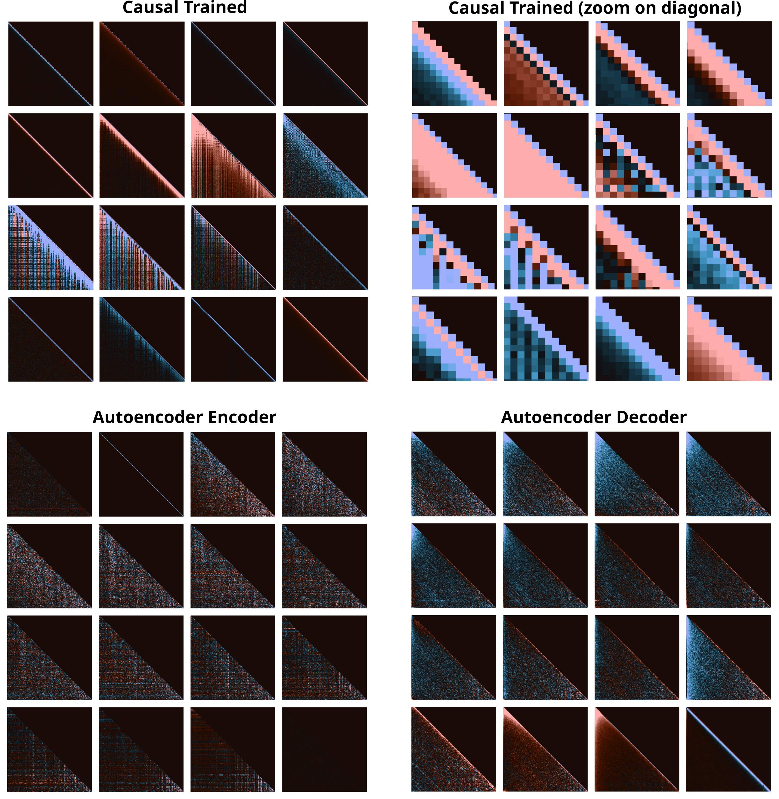
In the upper left, we find the entire 512x512 mixing matrix weights for all layers of a causal (next token prediction)-trained masked mixer, and in the upper right we zoom in on the main diagonal for a better understanding of the values therin.

The lower half of the above figure shows the weights for an autoencoder masked mixer, which are qualitatively substantially different.

Now that we have observed some token mixing matrix weights, we can attempt to capture some of the qualitative features of these transformations in order to design repeat mixer matrices that reflect these features. In the figure below, qualitative patterns of these matrices are labeled on somewhat higher-resolution representations of the token mixing matrices from layers 4-12 shown in the last figure.

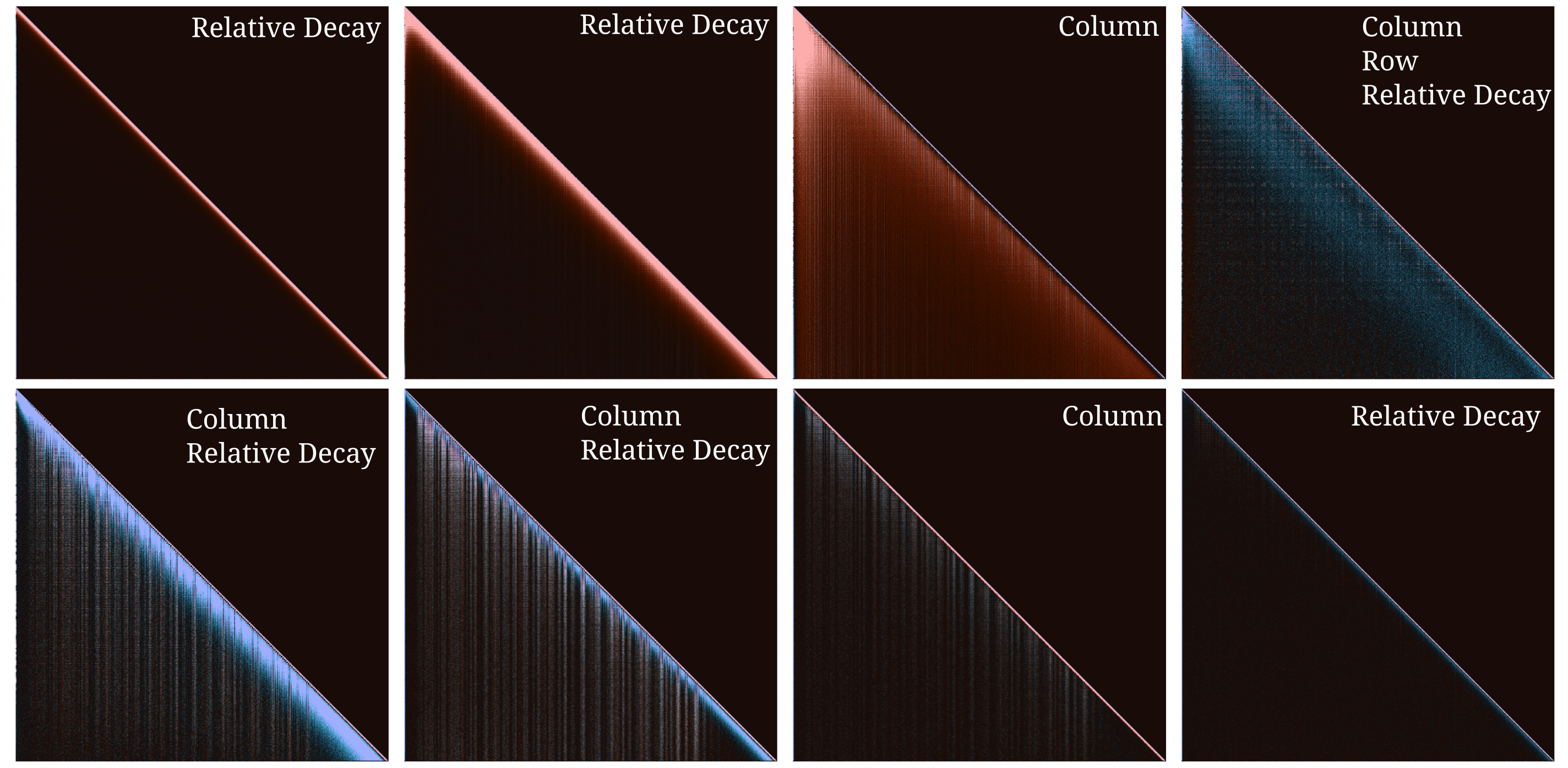
We find three features to be predominant: column lines, row lines, and weight decay with increased distance from the main diagonal. As lines of similar color and intensity indicate near-constant values, we can substitute constants for these by simply repeating a single value in the row or column orientation.

We have already explored row repeats and shown that these results in linear complexity models, but it is useful to observe that column repeats are as well. Consider the following:

\[\begin{pmatrix} \vert & \vert & \vert \\ Y_0 & Y_1 & Y_2 \\ \vert & \vert & \vert \end{pmatrix} = \begin{pmatrix} \vert & \vert & \vert \\ X_0 & X_1 & X_2 \\ \vert & \vert & \vert \end{pmatrix} \begin{pmatrix} a & b & c \\ 0 & b & c \\ 0 & 0 & c \end{pmatrix} + \begin{pmatrix} \vert & \vert & \vert \\ \beta_0 & \beta_1 & \beta_2 \\ \vert & \vert & \vert \end{pmatrix}\]

Now let’s solve for each output. It becomes clear that this is indeed a linear-complexity operation as well, and all we need to do is to cache the unscaled value of $X_0 + X_1 + X_2 + \cdots + X_n$ and rescale at each step.

\[Y_0 = a X_0 + \beta_0 \\ Y_1 = b X_1 + b X_0 + \beta_1 \\ Y_2 = c X_2 + c X_1 + c X_0 + \beta_2 \\ ... \\ Y_n = \alpha_n X_n + \beta_m + \alpha_n \sum_{m=0}^{m=n-1} X_m\]