Additivity and order

Probability

Imagine tossing a fair coin and trying to predict the outcome. There exists a 50% chance of success, but there is no way to know with any certainty what will happen. Now imagine tossing the coin thousands of times, and consider what you will be able to predict: each toss continues to be random and completely uncertain, so one’s ability to predict the outcome of each individual toss does not change. But now add the results of the tosses together, assigning an arbitrary value to heads and a different value to tails. As the number of individual coin tosses increases, one is better able to predict what value the sum will take. Moreover, if the same coin toss experiment is repeated many times (say repeating 1000 tosses 1000 times), we can predict what the sum of the tosses will be with even more accuracy.

Specifically, there are two possible outcomes for each toss (heads or tails) and so a binomial distribution is appropriate to model the expected value $E(X)$ after $n$ tosses as follows:

\[E(X) = n * p \\ E(X) = n * \frac{1}{2}\]

where $p$ is probability of the coin landing in a specific orientation, say heads.

The variance $V(X)$ approximates a binomial distribution centered around the expected value of each toss times the number of tosses.

\[V(X) = n * p (1-p) \\ V(X) = n \left( \frac{1}{2} \right) ^2\]

And the standard deviation is the square root of the variance,

\[\sigma = \sqrt{n \left( 1/2 \right)^2}\]

As n increases, $\sigma$ shrinks with respect to $E(V)$: after 100 tosses the standard deviation is 10% of the expected value, and after 1000 tosses the standard deviation is ~3% of the expected value, whereas after 10000 tosses the standard deviation is only 1% of the expected value. This is because $\sigma$ increases in proportion to the square root of $n$, whereas $E(V)$ increases linearly with $n$.

The second observation is perhaps more striking: the additive transformation on a coin toss leads to the gaussian distribution with arbitrarily close precision. Let’s simulate this so that we don’t have to actually toss a coin millions of times, assigning the value of $1$ to heads and $0$ to tails. We can compare the resulting distribution of heads to the expected normal distribution using scipy.stats.norm as follows:

import numpy
import matplotlib.pyplot as plt
from scipy.stats import norm

flips = 10
trials = 10
sum_array = []
for i in range(trials):
	s = 0
	for j in range(flips):
		s += numpy.random.randint(0, 2)
	sum_array.append(s)

variance = flips * (0.5) ** 2
y = numpy.linspace(0, flips, 100)
z = norm.pdf(y, loc=(flips/2), scale=(variance**0.5))

final_array = [0 for i in range(flips)]
for i in sum_array:
	final_array[i] += 1

fig, ax = plt.subplots()
ax.plot(final_array, alpha=0.5)
ax.plot(y, z*trials, alpha=0.5)
plt.show()
plt.close()

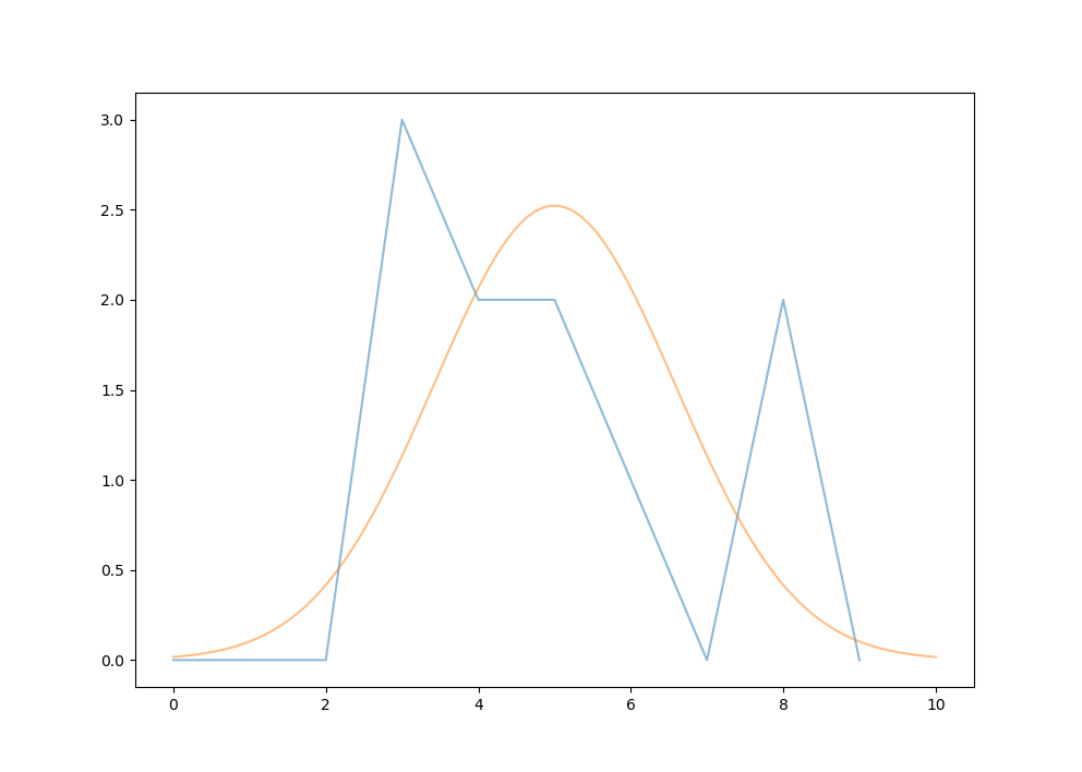
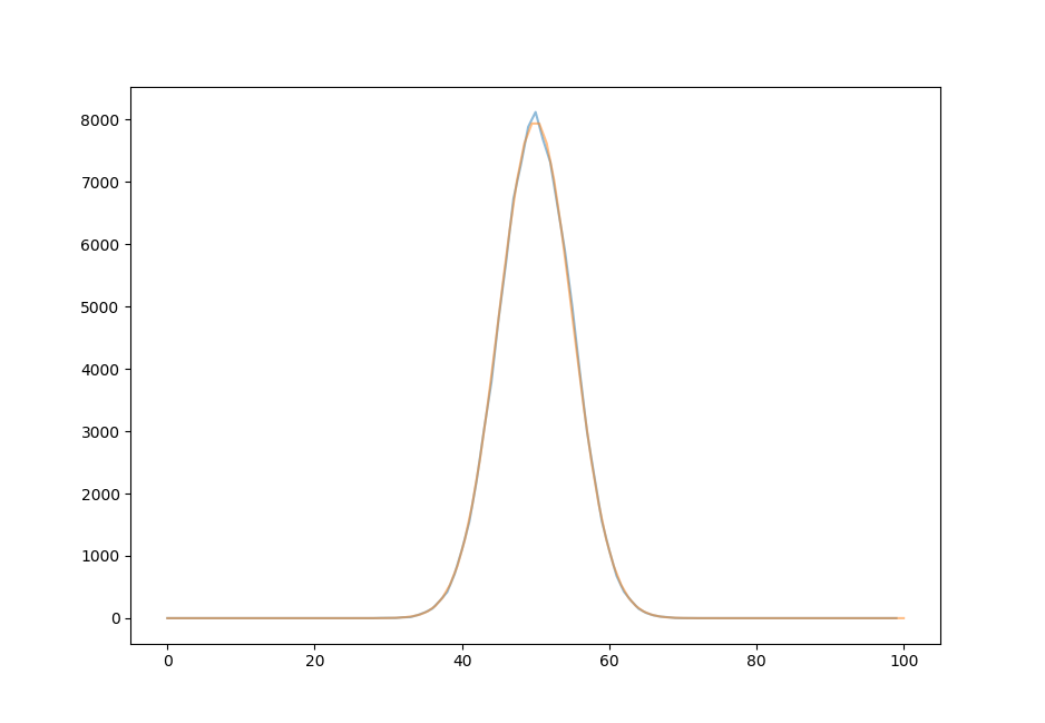
Let’s assign $n$ as the number of tosses for each experiment and $t$ as the number of experiments plotted. For 10 experiments ($t=10$) of 10 flips ($n=10$) each, the normal distribution (orange) is an inaccurate estimation of the the actual distribution (blue).

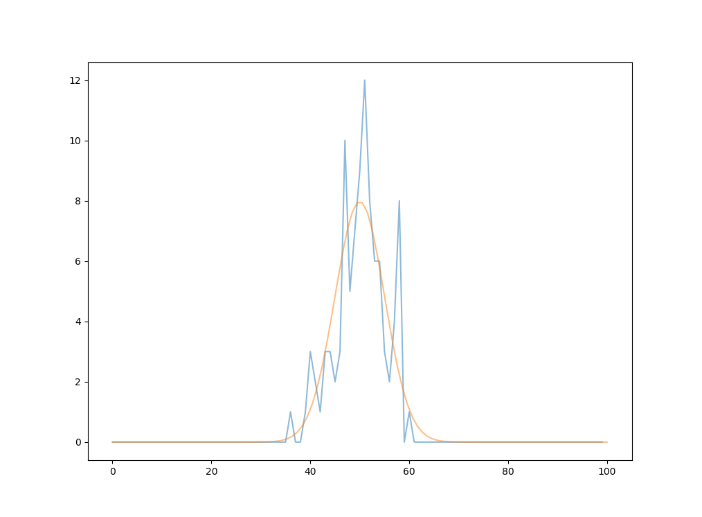
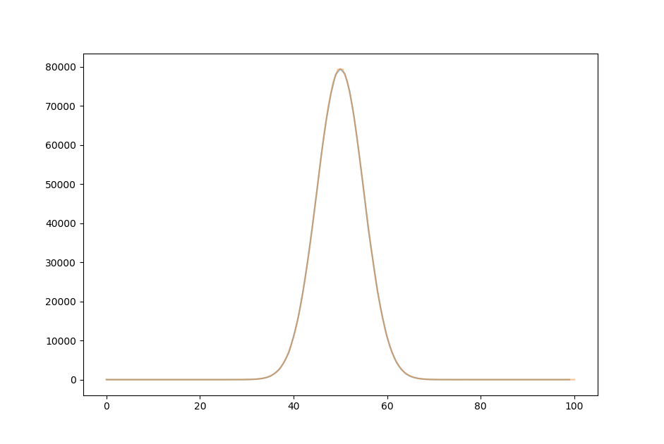
As we go from 100 tries of 100 tosses each to 1000000 tries of 100 tosses each, the normal distribution is fit more and more perfectly. For $n=100, t=100$,the distribution more closely approximates the normal curve.

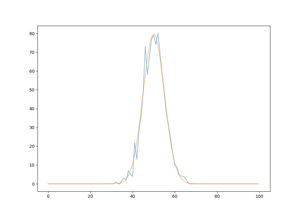
For $n = 100, t = 1000$,

for $n=100, t=1 * 10^4$,

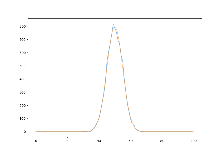
for $n=100, t=1 * 10^5$,

and for $n=100, t=1 * 10^6$, there is almost no discernable difference between the Gaussian curve centered on the expectation value of $50$ and the actual distribution.

Let’s take a moment to appreciate what has happened here: a random input can be mapped to a curve with arbitrary precision simply by adding outputs together. (Well, not completely random: digital computers actually produce pseudo-random outputs that are periodic with an exceedingly large interval. But we do not need to worry about that here, as our output number is far less than what would be necessary for repetition.)

This observation is general: individual random events such as a die roll or card shuffle cut are quite unpredictable, but adding together many random events yields a precise mapping to a gaussian curve centered at the expectation value. Each individual event remains just as unpredictable as the last, but the sum is predictable to an arbitrary degree given enough events. One way to look at these observations is to see that addition orders random events into a very non-random map, and if we were to find the sum of sums (ie integrate under the gaussian curve) then a number would be reached with arbitrary precision given unlimited coin flips and experiments.

Brownian motion

There is an interesting physical manifestation of the abstract statistical property of additive ordering: Brownian motion, the irregular motion of small (pollen grain size or smaller) particles in fluid. Thermal motions are often thought of as random or stochastic, meaning that they are described by probability distributions. Sush motions of fluid molecules add together on the surface of a larger particle to result in a non-differentiable path of that particle. Movement along this path is termed Brownian motion, after the naturalist Brown who showed that this motion is not the result of a biological process (although it very much resembles the paths taken by small protists living in pond water).

In three dimensions, Browniam motion leads to a movement away from the initial particle position. The direction of this movement is unpredictable, but over many experiments (or with many particles underging brownian motion at once), the distances of the particles away from the initial point together form a Gaussian distribution (see here for a good summary of this). Regardless of the speed or trajectory of each individual particle undergoing Brownian motion, an ensemble that start at the same location form a Gaussian distribution with arbitrary accuracy, given enough particles.

White and fractional noise

Noise may signify the presence of sound, or it may mean any observation that is not classified as a signal. Both meanings are applicable here. White noise is defined as being frequency-independent: over time, neither low nor high frequencies are more likely to be observed than the other. Fractional noise is defined here as any noise that is inversely frequency-dependent: lower frequency signal occurs more often than higher frequency signal. Inverse frequency noise is also called pink or $1/f$ noise.

White noise is unpredictable, and ‘purely’ random: one cannot predict the frequency or intensity of a future signal any better than by chance. But because fractional noise decays in total intensity with an increase in frequency, this type of noise is not completely random (meaning that it is somewhat predictable). Consider one specific type of fractional noise, Brown noise, which for our purpose is characterized by a $\frac{1}{f^n}, \; n > 0$ frequency vs. intensity spectrum. This is the noise that results from Brownian motion (hence the name). It may come as no surprise that another way to generate this noise is to integrate (sum) white noise, as the section above argues that Brownian motion itself acts to integrate random thermal motion.

As noted by Mandelbrot and Bak, fractional noise results from fractal objects as they change over time. Brownian noise coming from Brownian motion is simply a special case of this more general phenomenon: Brownian motion traces out fractal paths. These paths are self-similar in that very small sections of the path resemble much larger sections, not that smaller portions exactly match the whole as is the case for certain geometric fractals. This type of self-similarity is sometmies called statistical self-similarity, and is intimately linked to the property this motion exhibits of being nowhere-differentiable. For more about fractals, see here.

In general terms, Brownian motion is a fractal because it appears to trace paths that are rough and jagged at every scale until the atomic, meaning that at large scales the paths somewhat resemble the Weierstrauss function above. Now imaging trying to measure the length of such a shape: the more you zoom in, the longer the measurement is! Truly nowhere-differentiable paths are of infinite length and instead can be characterized by how many objects (a box or sphere or any other regular shape) it takes to cover the curve at smaller and smaller scales (either by making the shapes themselves smaller or by making the curve larger). The ratio of the logarithm of the change in the number of objects necessary for covering the curve (a fraction) divided by the logarithm of the change in scale is the counting dimension. Equivalently,

\[D = \frac{log(N)}{log(1/r)} \\ N = \left( \frac{1}{r} \right) ^D \\\]

where $D$ is the fractal dimension, $N$ is the ratio of the number of objects required to cover the curve, and $1/r$ is the change in scale expressed as a fraction. Note that this is equivalent to the equation for fractional (Brownian) noise,

\[I = \left( \frac{1}{f} \right) ^n\]

where the number of objects required to cover the curve N is eqivalent to the signal intensity I, the radius of the objects r is equivalent to the frequency f, and the dimension D is equivalent to the noise scaling factor n.

If the fractal dimension is larger than the object’s topological dimension, it is termed a fractal. For very rough paths, an increase in scale by, say, twofold leads to a larger increase in the number of objects necessary to cover the path because the path length has increased relative to the scale. Brownian trails in two dimensions have a fractal dimension of approximately $2$, meaning that they cover area even though they are topologically one-dimensional.

Gambler’s fallacy

Statistical distributions of the natural world rarely conform to Gaussian distributions. Instead, rare events are often overrepresented: the more data that is obtained, the larger the standard deviation describing those observations. This is equivalent to the fractal noise mentioned above, where uncommon events (low frequency signal) are over-represented compared to the expected value for these events if modeled with white noise. This implies that truly independent samples are rare, a conclusion that is often in agreement with experimentation. For example, the weather a place receives from one day to the next is not completely independent, as a downpour one day will lead to greater humidity in the hours following, which necessarily affects the weather of the hours following.

The gambler’s fallacy may be defined as a tendancy to assume that events are not independent. In light of the ubiquity of fractal noise and scarcity of white noise in the natural world, it may be that the gambler’s fallacy is actually a more accurate interpretation of most natural processes than one assuming independent events.

Nonlinear statistics

Additivity is usually assumed in the calculation of expectated values:

\[E(A + B) = E(A) + E(B) \\ if \; E(A) \; \bot \; E(B)\]

or the expected value of event A or B is the same as the expected value of A plus the expected value of B. Additivity is a given for independent events. Additivity also holds for pseudoindependent events, meaning those that are dependent but not non-randomly dependent. When events are non-randomly dependent, additivity is no longer valid because a change in the expectation value of one event could change the expectation value of the other:

\[E(A + B) \neq E(A) + E(B) \\ if \; \lnot E(A) \; \bot \; E(B)\]

Markov processes attempt to model non-random dependencies by providing each state with a separate probability rule, and then by applying standard linear statistical rules to each separate state. This is similar to the decomposition of a curve into many small lines and is a practical way of addressing simpler probability states such as those that exist while playing cards, but is extremely difficult to use to model states where each decision leads to exponentially more states in the future (as is the case for chess, where one starting configuration leads to $10^{46}$ possibilities for future ones).

It may instead be more effective to consider a nonlinear model of statistics in which additivity is not assumed (meaning that the expected value of one variable may affect the expected value of another in a nonrandom (and noncomplementary) way. One could imagine a Markov chain-like graph in which the state probabilites continually updated depending on the path to each state.

Randomized fractals

One example of organization is found in randomized fractals. These are shapes that can be obtained by from random (pseudorandom, as no digital computer is capable of truly random number generation) inputs that are restricted in some way. Take the Sierpinski triangle:

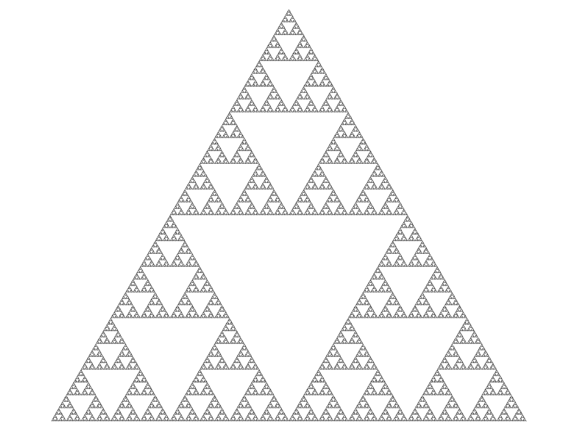
This fractal may be constructed in a deterministic fashion by instructing a computer to draw exactly where we want it to using recursion on a base template consisting of seven line segments with exact angles between them (for more on exactly how to draw this fractal, see here).

The Sierpinski triangle can also be constructed using random inputs in a surprising way: take three points that are the edges of an equilateral triangle and add an initial point somewhere in this triangle. Assign two numbers on a dice to each vertex, roll the dice, and move half way towards the vertex indicated by the dice and repeat. This can be done in python as follows:

a = (-400,-300)
b = (0, 300)
c = (400, -300)

def randomized_sierpinski(steps, a, b, c):
	'''
	A function that draws the sierpinski triangle using random.randint, accepts arguments 'steps' (int)
	for the number of points to plot and 2D vertex points a, b, and c (tuples) as the corners of an 
	equilateral triangle.
	'''
	for i in range(steps):
		pos = [j for j in turtle.pos()] # find current position

		n = random.randint(0, 6) # dice roll
		turtle.pu()
		# move half way towards the vertex indicated by the dice roll
		if n < 2:
			turtle.goto((pos[0]+a[0])/2, (pos[1]+a[1])/2)

		elif n >= 4:
			turtle.goto((pos[0]+b[0])/2, (pos[1]+b[1])/2)

		else:
			turtle.goto((pos[0]+c[0])/2, (pos[1]+c[1])/2)

		turtle.pd()
		# skip the first 100 rolls 
		if i > 100:
			turtle.forward(0.5)

One might think that this procedure would result in a haze of random points in the triangle. Indeed, if the verticies of a square are used instead of a triangle then the plotted points occupy random positions in this square and do not make a pattern. But in a triangle, the following shape is made:

Guessing where the next point will land is not possible, but as more and more iterations are made each iteration comes arbitrarily close to the Sierpinski triangle. This occurs regardless of where the initial point is located! The points, when added togather, approximate the intricate structure of a fractal.

For a more dramatic example of the organizing effect of a decrease in distance travelled towards the chosen vertex on each iteration, observe what happens when we go from $d = 1 \to d = 1/4$, or in other words when we go from $(x, y) + (v_x, v_y)$ to $((x, y) + (v_x, v_y))/4)$ on each iteration:

A similar process can be used to make a Sierpinski carpet. The idea is to specify the location of four verticies of a rectangle as $a, b, c, d$. Each iteration proceeds as above, except that the pointer only moves $1/3$ the distance to the vertex chosen by the random number generator.

from turtle import *
import turtle
import random

a = (-500,-500)
b = (-500, 500)
c = (500, -500)
d = (500, 500)
div = 3
def randomized_sierpinski(steps, a, b, c, d, div):
	for i in range(steps):
		pos = [j for j in turtle.pos()]

		n = random.randint(0, 8)
		turtle.pu()
		if n < 2:
			turtle.goto((pos[0]+a[0])/div, (pos[1]+a[1])/div)

		elif n >= 6:
			turtle.goto((pos[0]+b[0])/div, (pos[1]+b[1])/div)

		elif n < 6 and n >= 4:
			turtle.goto((pos[0]+c[0])/div, (pos[1]+c[1])/div)

		elif n < 4 and n >= 2:
			turtle.goto((pos[0]+d[0])/div, (pos[1]+d[1])/div)

		turtle.pd()
		if i > 100:
			turtle.forward(0.5)

And the setup for viewing the resulting carpet from $d=1 \to d=1/4$ is

...
div = 1
...
for i in range(300):
	turtle.hideturtle()
	turtle.speed(0)
	turtle.delay(0)

	turtle.pensize(2)
	width = 1900
	height = 1080
	turtle.setup (width, height, startx=0, starty=0)

	print (i)
	randomized_sierpinski(5000, a, b, c, d, div + i/100)
	turtle_screen = turtle.getscreen()
	turtle_screen.getcanvas().postscript(file="randomized_sierpinski{0:03d}.eps".format(i), colormode = 'color')
	turtle.reset()

which results in a Sierpinski carpet.

Irrationals are not closed under addition

Here it is established for a certain class of dynamical equation that periodic maps exist in a bijective correspondence with the rational numbers, and that aperiodic maps correspond to irrational numbers $\Bbb I$. What happens if we add together multiple aperiodic maps: can a periodic map ever result? Defining addition on maps here could be simply a composition of one map with another.

$\Bbb I$ is not closed under addition (or subtraction). For example, $x_1 = 1 + \pi$ is irrational and $x_2 = 2 - \pi$ is irrational but $y = x_1 + x_2 = 3$ which is rational. By equivalence two aperiodic maps may be added together to yield a periodic one, according to the method of digits (see the link in the last paragraph).

But note that $\Bbb Q$ is closed under addition (and subtraction), meaning that two rationals will not add to yield an irrational. This means that, given a set $S$ of numbers in $\Bbb R$, addition may convert elements of $S$ from irrational to rational. For a set of trajectory maps $M$, addition may lead to the transformation of aperiodic trajectories to periodic.

Aside: quantum mechanics and non-differentiable motion

The wave-like behavior of small particles such as photons or electrons is one of the fundamnetal aspects of the physics of small objects. Accordingly, the equations of quantum mechanics have their root in equations describing macroscopic waves of water and sound. Now macroscopic waves are the result of motion of particles much smaller than the waves themselves. As quantum particles are well-described by wave equations, it seems logical to ask whether or not these particles are actually composed of many smaller particles in the same way macroscopic waves are.

As a specific example of what this would mean, imagine a photon as a collection of particles undergoing browninan motion for a time that is manifested by the photon’s wavelength: longer wavelengths mean more time has elapsed whereas smaller wavelengths signify less time. When a photon is detected, it forms a Gaussian distribution and this is exactly the pattern formed by a large collection of particles undergoing Brownian motion for a specified time. The same is true for any small particle: the wavefunctions ascribed to these objects may be represented as Brownian motion of many particles.

If this seems strange, consider that this line of reasoning predicts that the paths of small particles, as far as they can be determined, are non-differentiable everywhere, just as the path of a particle undergoing Brownian motion is. In the path integral approach to quantum events, this is exactly what is assumed and the mathematics used to make sense of quantum particle interactions (uncertainty relations etc.) is derived from the mathematics used to understand Brownian motion of macroscopic particles. This math is tricky because nowhere-differentiable motion is not only poorly understood in a simple form by calculus, but the paths themselves of such particles are infinitely long, leading to a number of paradoxes.

The similarities that exist between how quantum particles behave and how macroscopic particles behave when undergoing Brownian motion suggests that we consider the possibility of small particles existing in a similar environment to macroscopic ones in fluid.