Fractal Geometry

Images of nonlinear dynamical systems are typically fractals. Here we explore the origin and meaning of this term.

Origin and Cantor sets

The term Fractal was chosen by Mandelbrot (after the Latin Fractus) to signify irregular, fragmented objects. These often but do not necessarily have a fractional scaling dimension, and the surface of these objects is non-differentiable. Spectacular examples of fractals such as the Julia and Mandelbrot sets are often brought to mind when one thinks of fractals, but they are far older and richer than these examples alone. Nearly a century before the word fractal had been invented, the foundations for this branch of math were established and are here roughly detailed.

In the late 19th century Cantor founded set theory, a study of abstract collections of objects and the relations between these collections. Other pages in this website make use of set theory, and for a good background on the subject see “Naive set theory” by Halmos. From set theory, we find fascinating conclusions that lay a foundation for fractal geometry, so to understand the latter it is best to examine a few key aspects of the former.

Surprising results abound in set theory, but one of the most relevant here pertains to counting how many elements a set has. It turns out that not all infinite sets are equal: there are as many elements of the set of positive numbers as there are rational numbers (an infinite amount of each) but there are far more elements of the set of real numbers than either of the other two sets. The elegant diagonal proof for this is worth viewing elsewhere, as it reappears again in other forms (in Turing’s computability theories, for example).

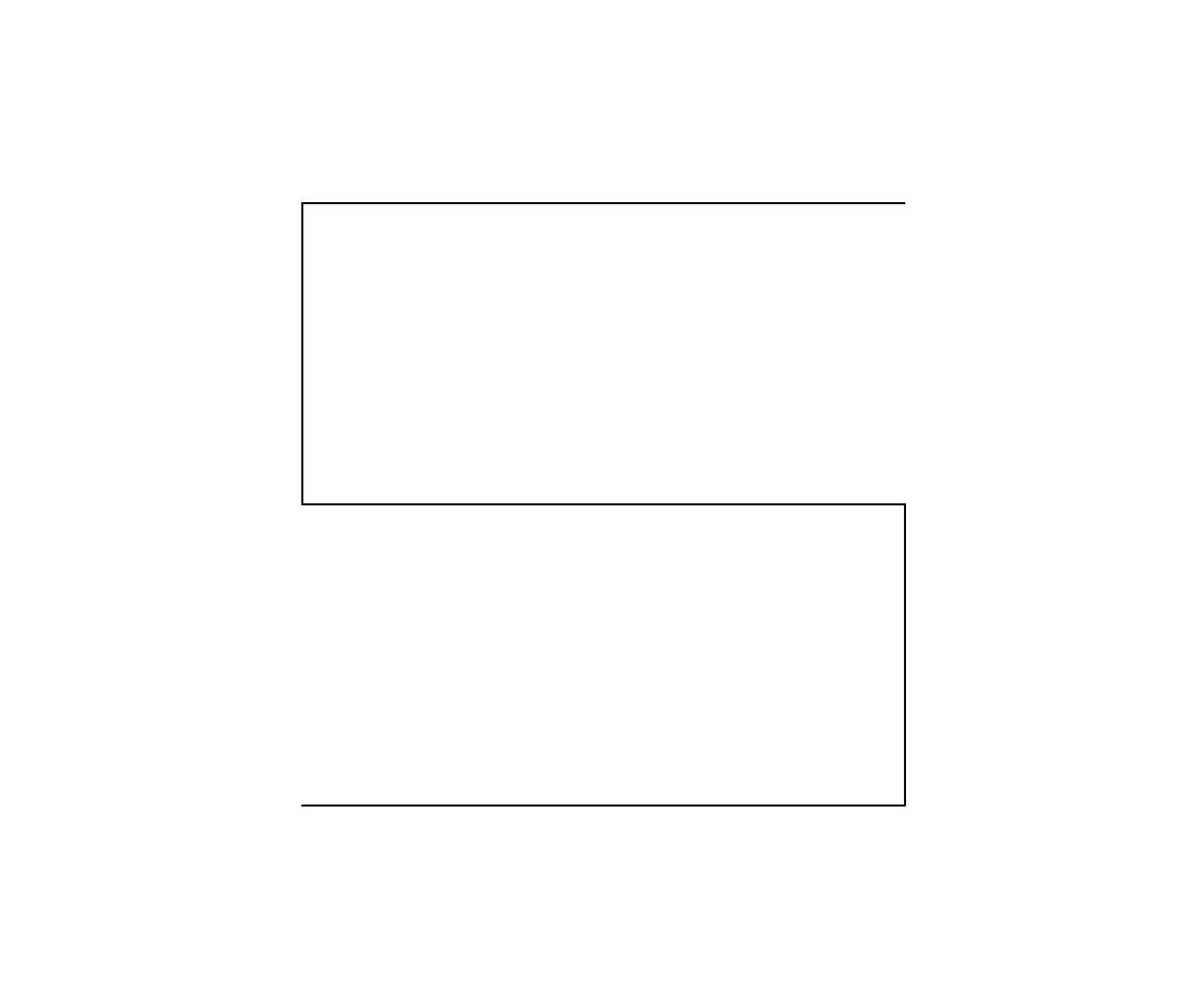
A particularly interesting set is known as the middle thirds Cantor set $C$. This set will be considered in some detail because it illustrates many of the most important aspects of fractals but is relatively simple, existing on a line. $C$ is made as follows: take the closed interval on the reals $[0, 1]$ and remove from this an open interval of the middle third, that is, $[0, 1] - (1/3, 2/3)$.

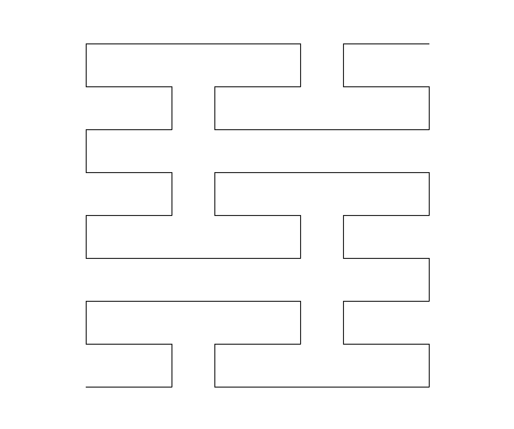
Now repeat this process for each remaining closed intervals,

and again

and so on ad infinitum. $C$ is the set of numbers that remains after an infinite number of these steps. This set is remarkable: after n steps of removing the inner third, $(\frac{2}{3})^n$ total length remains. Therefore $C$ has $0$ total length: $(2/3)^n \to 0 \; as \; n \to \infty$. If it has $0$ length, does $C$ have any points? It does indeed, just as many points as the original closed interval $[1,0]$! The set is totally disconnected (no point touches any other point) and perfect (every point is a limit of another set of points in $C$).

This set can be drawn with Turtle, a Python programming library that was designed to help teach programming in a visual way. It turns out to be quite capable of intricate fractal drawings as well.

from turtle import *
import turtle

def cantor_set(size, recursive_steps):
	if recursive_steps > 0:
		cantor_set(size/3, recursive_steps-1)

		turtle.pu(), turtle.forward(size), turtle.pd()
		cantor_set(size/3, recursive_steps-1)

	else:
		turtle.color('red'), turtle.forward(size)
		turtle.pu(), turtle.forward(size), turtle.pd()
		turtle.color('blue'), turtle.forward(size)


for i in range(300):
	turtle.hideturtle()
	turtle.speed(0), turtle.delay(0)
	turtle.pensize(4)
	turtle.setup (width=1900, height=1080, startx=0, starty=0)
	turtle.pu(), turtle.goto(-800, 0), turtle.pd()

	cantor_set(500 * (2**(i/30)), 4 + i // 30)
	turtle_screen = turtle.getscreen()
	turtle_screen.getcanvas().postscript(file="cantor_set{0:03d}.eps".format(i))
	turtle.reset()

The .eps files generated by this program are vector images, and to make a video conversion to a fixed size .png or .jpg type file is useful. Fortunately the Python Image Library has the wonderful ability to detect and reformat all kinds of image types! I used the following program to convert .eps to .png files:

from PIL import Image
import os

 # insert path here
path = '/home/bbadger/Desktop/' 

files = os.listdir(path)

for i in range(0, len(files)):
	string = str(i)
	while len(string) < 3:
		string = '0' + string
	try:
		eps_image = Image.open('cantor_set' + string + '.eps') # input names here
	except:
		break
	eps_image.load(scale=2)   
	eps_image.save('cantor{0:03d}.png'.format(i)) # output names here

After compiling these .png images into an mp4 using ffmpeg in bash

(base) bbadger@bbadger:~$ ffmpeg -f image2 -r 30 -pattern_type glob -i '*.png' cantor_zoom.mp4

the video can be viewed and edited. Here it is as a .gif (ffmpeg can convert directly into gifs simply by changing the extension name to cantor_zoom.gif, but these are uncompressed and can be quite large files)

As the number of recursive calls increases, the Cantor set becomes invisible. This should not come as a surprise, being that it is of measure $0$ as $n \to \infty$. Thus in order to obtain a viewable map with more recursive steps, vertical lines are used to denote the position of each point in the set. The following program accomplishes this by drawing alternating red and blue vertical lines at the start of where each set interval (at any given step) begins and so is only accurate with a relatively large value for the starting number of recursions (>4). A black background is added for clarity, and once again the number of recursive steps increases with scale to maintain resolution.

Starting at the 5th recursive level (code available here) and adding a recursion every 30 frames, we have

Now this is one particular example of a Cantor set, but there are others: one could remove middle halves instead of thirds etc. The general definition of a Cantor set is any set that is closed, bounded, totally disconnected, and perfect. The general Cantor set $C$ is a common occurence in nonlinear maps. The period doubling in the logistic map forms a Cantor set, although this is not a middle thirds set as seen above

as well is in the henon map.

Space filling curves

What is the dimension of the Cantor set? Finite collections of points are of dimension $0$, whereas lines are of dimension $1$. $C$ is totally disconnected and therefore would seem to be $0$ dimensional, and yet it is an infinite collection of points that are bounded to a specific region. Thus $C$ has characteristics of both zero and one dimensions. Do any other curves also exhibit properties of multiple dimensions?

One can defined fractals as objects that exhibit properties of multiple dimensions, and in that respect every image on this page is an example of a curve that answers this question. But before exploring those, it may be useful to view some extreme cases: curves (1-dimensinal objects) that fill space (2 dimensions). One of the first such curves to be discovered to do this by Peano in the late 19th century can be described in python as follows

ls = [90, -90, -90, -90, 90, 90, 90, -90, 0]
def peano_curve(size, recursive_steps, ls):
	if recursive_steps > 0:
		for i in range(len(ls)):
			peano_curve(size, recursive_steps-1, [i for i in ls])
			turtle.left(ls[i])
	else:
		turtle.forward(size)

where recursive_steps goes to infinity. To understand how this fills space, observe the base case:

and the first recursive step, where each line segment of the curve above is replaced with a smaller version of the whole curve:

After a few more recursive steps (only 5 in total!) , the present resolution is no longer able to differentiate between one line and another and we have achieved something close to a space-filling curve.

This curve fills space but crosses over itself. The following is another space filling curve from Peano that does not self-cross but is more difficult to draw. The L -system, named after its discoverer Lindenmayer, is a very useful system for characterizing the generation of more complex recursive structures. For a good overview of this system complete with examples, see here. The Peano curve may be defined in the L-system by the sequences X = 'XFYFX+F+YFXFY-F-XFYFX', Y = 'YFXFY-F-XFYFX+F+YFXFY' where X and Y are separate recursive sequences, ‘+’ signifies a turn left by 90 degrees, ‘-‘ a turn right 90 degrees, and ‘F’ signifies a movement forward. This can be implemented in python by interpreting each L-system element separately as follows:

def peano_curve(size, steps, orientation):
	X = 'XFYFX+F+YFXFY-F-XFYFX'
	Y = 'YFXFY-F-XFYFX+F+YFXFY'
	l = r = 90

	if steps == 0:
		return

	if orientation > 0:
		for i in X:
			if i == 'X':
				peano_curve(size, steps-1, orientation)
			elif i == 'Y':
				peano_curve(size, steps-1, -orientation)
			elif i == '+':
				turtle.left(90)
			elif i == '-':
				turtle.right(90)
			else:
				turtle.forward(size)

	else:
		for i in Y:
			if i == 'X':
				peano_curve(size, steps-1, -orientation)
			elif i == 'Y':
				peano_curve(size, steps-1, orientation)
			elif i == '+':
				turtle.left(90)
			elif i == '-':
				turtle.right(90)
			else:
				turtle.forward(size)

The base case

and first recursion

at the fifth recursion level,

As is the case in the first Peano curve, the true space-filling curve is the result of an infinite number of recursive steps. This means that the curve is also infinitely long, as the length grows upon each recursive step. Infinite length is a prerequisite for any space-filling curve.

Note that both of these curves are nowhere-differentiable: pick any point on the curve, and it is an angle (a 90 degree angle to be precise) and as angles are non-differentiable, the curve is non-differentiable.

These curves map a line of infinite length to a surface, and the mapping is continuous. But importantly, this mapping is not one-to-one (injective): multiple points on the starting line end up at the same spots in the final surface. In fact no injective mapping exists between one and two dimensions exists, and a geometric proof of this in the second Peano curve is as follows: observe the point at the upper right corner of the curve $p_1$ and the point directly below it $p_1$ to be $p_2$. Upon each recursion $r$, the distance between these points is divided by 3 such that

\[d(p_1, p_2)_{r+1} = \frac{d(p_1, p_2)_{r}}{3} \\ \; \\ \frac{1}{3^n} \to 0 \; as \; \; n \to \infty \\ \; \\ d(p_1, p_2) \to 0 \; as \; \; r \to \infty\]

Now the true Peano curves are infinitely recursive, therefore this the distance between these points is 0 and therefore $p_1$ and $p_2$ map to the same point in two dimensional space, making the Peano curve a non-injective mapping.

Imagine moving along the surface created by either peano curve. An arbitrarily small movement in one direction along this surface does not necessarily lead to a small movement along the curve itself. Indeed it can be shown that any mapping from two to one dimensions (which could be considered to be equivalent to the definition of a space filling curve) is nowhere-continuous if the mapping is one-to-one and onto. For some interesting repercussions of this on machine learning methods such as neural networks, see here.

Fractals as objects of multiple dimensions

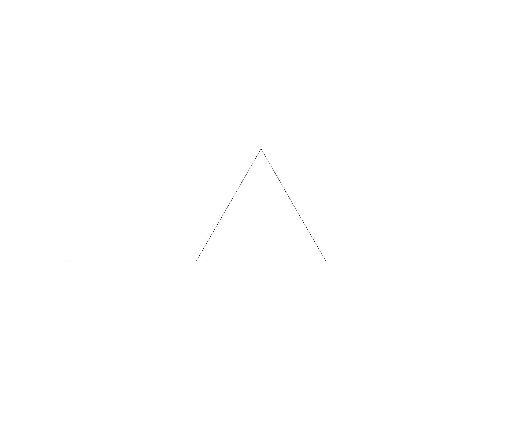
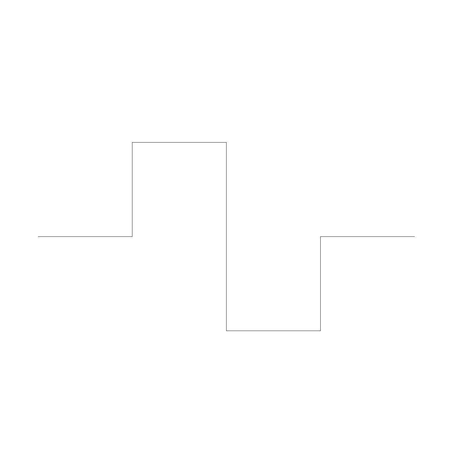
The Koch curve may be drawn as follows

ls = [60, -120, 60, 0]
def koch_curve(size, recursive_steps, ls):
	if recursive_steps > 0:
		for i in range(len(ls)):
			koch_curve(size, recursive_steps-1, [i for i in ls])
			turtle.left(ls[i])

	else:
		turtle.forward(size)

The curve starts as

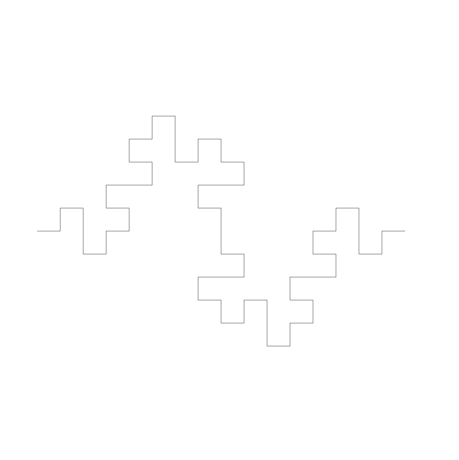
and at each recursion, each line segment is divided into parts that resemble the whole. At the 2nd,

3rd,

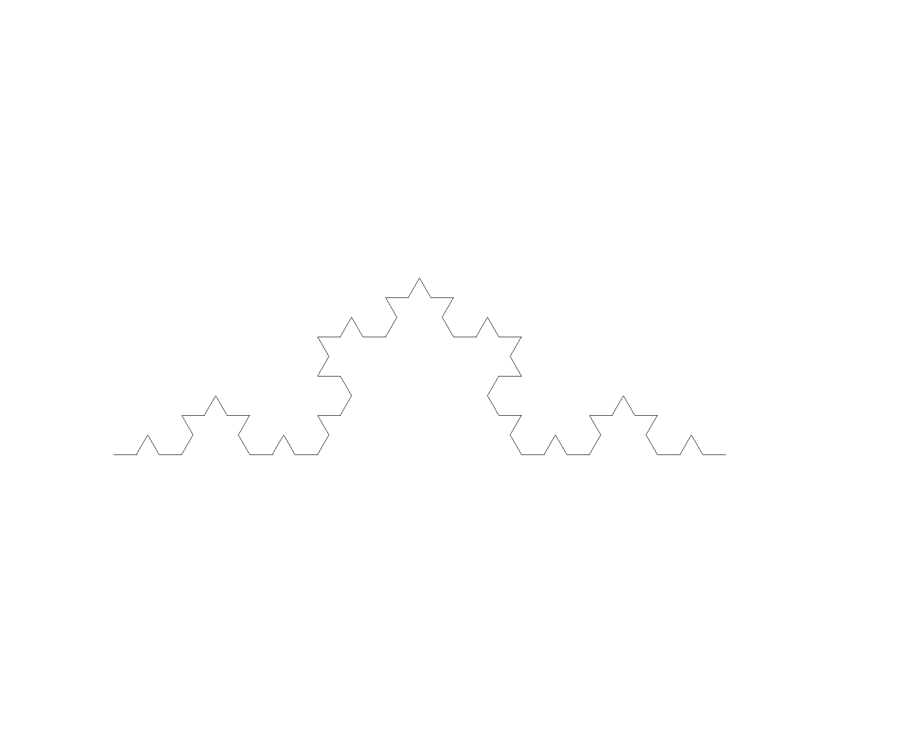
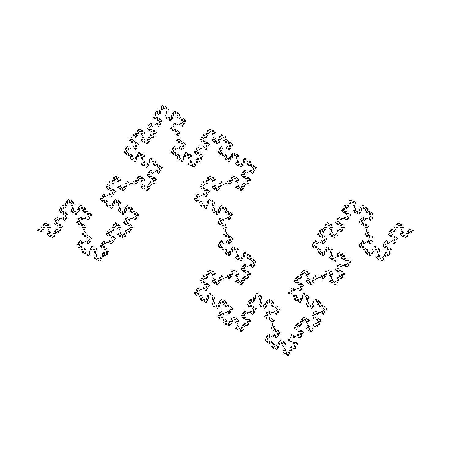
and 6th recursion:

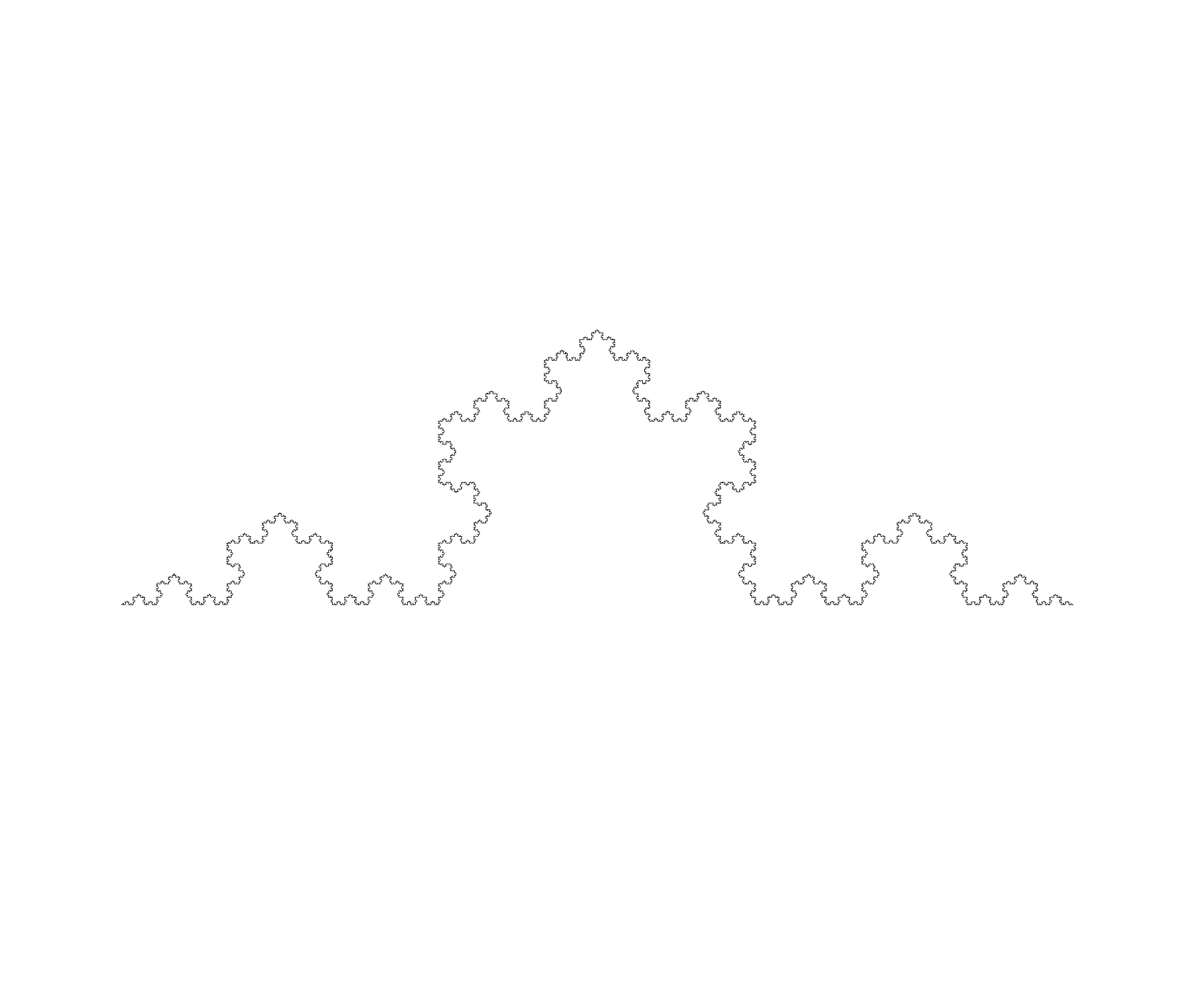
Now this curve evidently does not cover the plane like the Peano curves. But the curve does seem ‘fuzzy’, and that it might cover at least part of the plane. In this respect, it seems to be partway between dimensions. Is this the case?

A better understanding comes from the similarity dimension, which is equivalent to the Hausdorff dimension for the following self-similar objects. First note that Euclidean objects like a point, line, or surface have the same topological dimension as their similarity dimension: a point cannot be subdivided ($n^0 = 1$), a line of length n can be subdivided into $n^1 = n$ pieces, and a surface square of length n can be subdivided into $n^2$ pieces. Now note that the Koch curve may be subdivided into four equal pieces, and that these pieces are $1/3$ the length of the total curve. It’s similarity dimension is therefore

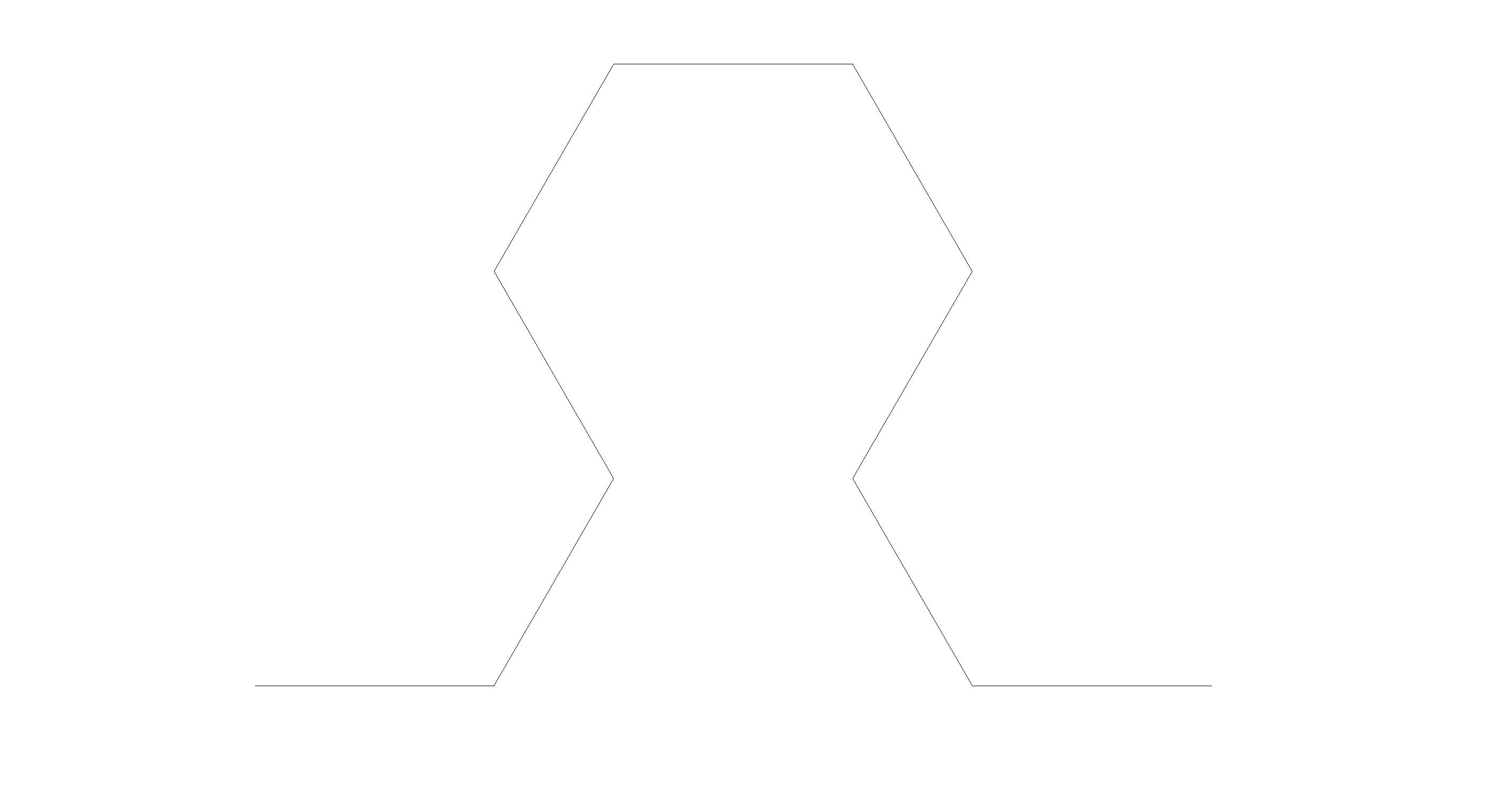
\[D = \frac{\log N}{\log (1/r)} \\ \; \\ D = \frac{\log 4}{\log 3} \approx 1.2618\]

Now consider the following curve, known as the quadric Koch curve:

ls = [90, -90, -90, 0, 90, 90, -90, 0]
def quadric_koch_curve(size, recursive_steps, ls):
	if recursive_steps > 0:
		for i in range(len(ls)):
			quadric_koch_curve(size, recursive_steps-1, ls)
			turtle.left(ls[i])

	else:
		turtle.forward(size)

The curve starts as follows:

in the first recursion,

and after 5 recursive levels,

Let’s calculate this curve’s similarity dimension: there are 8 pieces that are smaller versions of the whole curve, and these pieces are $1/4$th the length of the whole so therefore

\[D = \frac{\log N}{\log (1/r)} \\ \; \\ D = \frac{\log 8}{\log (4)} = 1.5 \\\]

This curve has a slightly larger dimension than the other Koch curve, which could be interpreted as being that this curve is closer to a surface than the first Koch curve. Visually, this results in the appearance of a rougher line, one that appears to cover more area than the first. How long are these curves? Each recursion adds length so just like the space-filling curves, the total length is infinite.

We can also calculate the dimension of the Cantor set. There are 2 collections of points that are identical in structure to the entire collection, which we can call L and R. These collections take up a third of the original interval, and so the dimension of $C$ is

\[D = \frac{\log N}{\log (1/r)} \\ \; \\ D = \frac{\log 2}{\log (3)} \approx 0.631\]

which is somewhere between $0$ and $1$, and this matches the observations that $C$ exhibits properties of both $0$ and $1$ dimensional objects.

Fractals are defined as shapes that have a Hausdorff dimension greater than their topological dimension. For the shapes presented on this page, Hausdorff and scaling dimensions are equal. Thus the curves in this section are all fractals, as are the Cantor set and both space-filling Peano curves.

More Selfsimilar fractals

The Sierpinski triangle (which will resemble a triforce for those of you who played Zelda) is one of the most distinctive fractals presented in the book. There are two orientations the curve takes, which means that the drawing proceeds as follows:

ls = [60, 60, -60, -60, -60, -60, 60, 60, 0]
def sierpinski_curve(size, recursive_steps, ls):
	if recursive_steps == 0:
		turtle.forward(size)
	else:
		for i in range(len(ls)):
			if i % 2 == 0:
				sierpinski_curve(size, recursive_steps-1, [i for i in ls])
				turtle.left(ls[i])
			else:
				sierpinski_curve(size, recursive_steps-1, [-i for i in ls])
				turtle.left(ls[i])

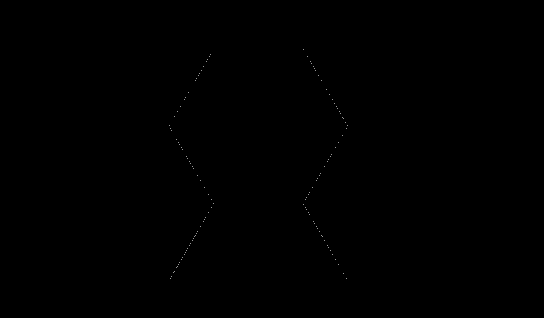
The starting point is

and each line becomes as smaller version of the whole upon the first recursion

And after a few more recursive levels, the following curve is produced:

The following fractal is reminiscent of the appearence of [endocytosis] in cells

def endocytic_curve(size, recursive_steps):
	if recursive_steps > 0:
		for angle in [60, -60, -60]:
			turtle.left(angle)
			endocytic_curve(size, recursive_steps-1)
		turtle.left(60)
	else:
		turtle.forward(size)

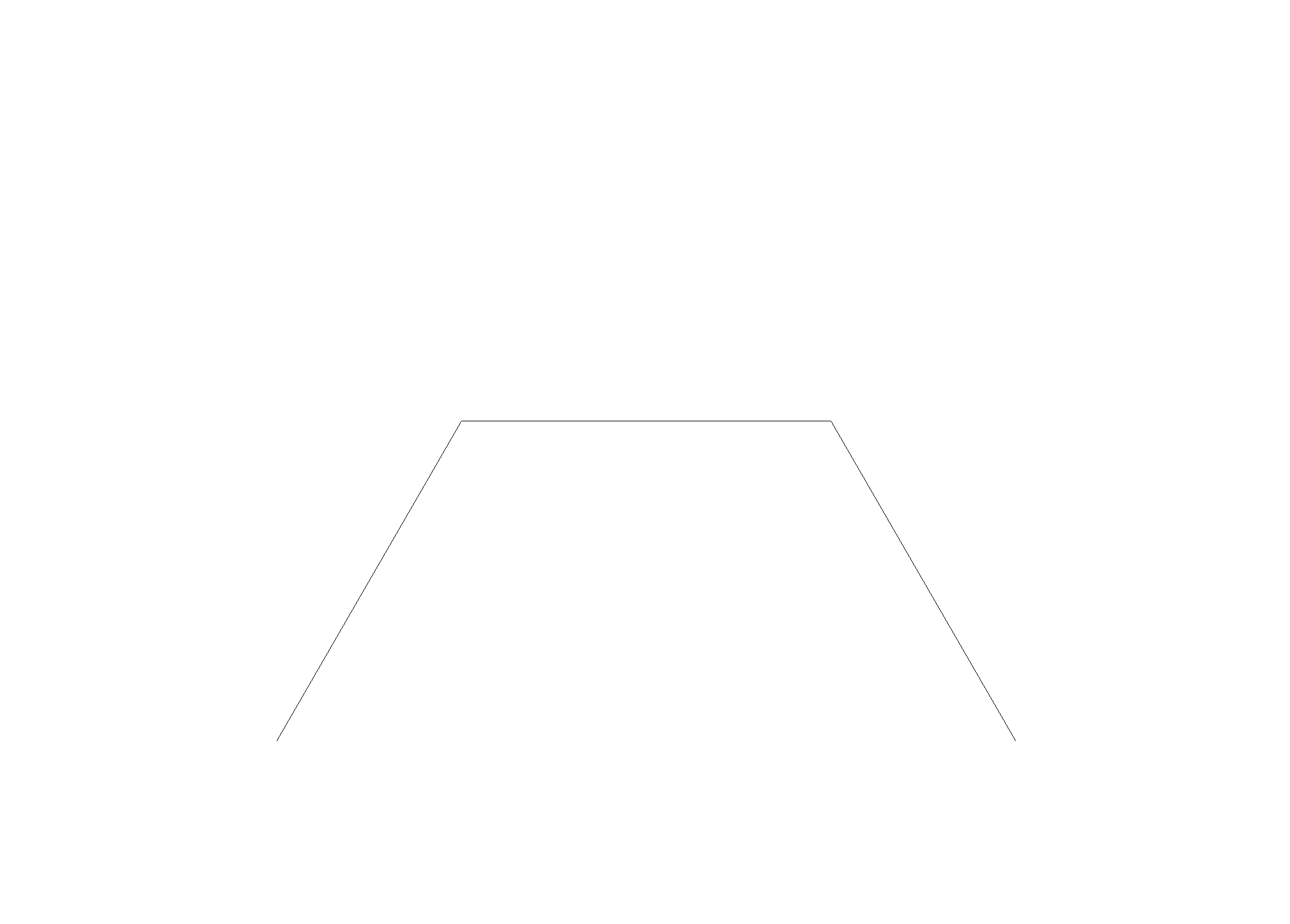
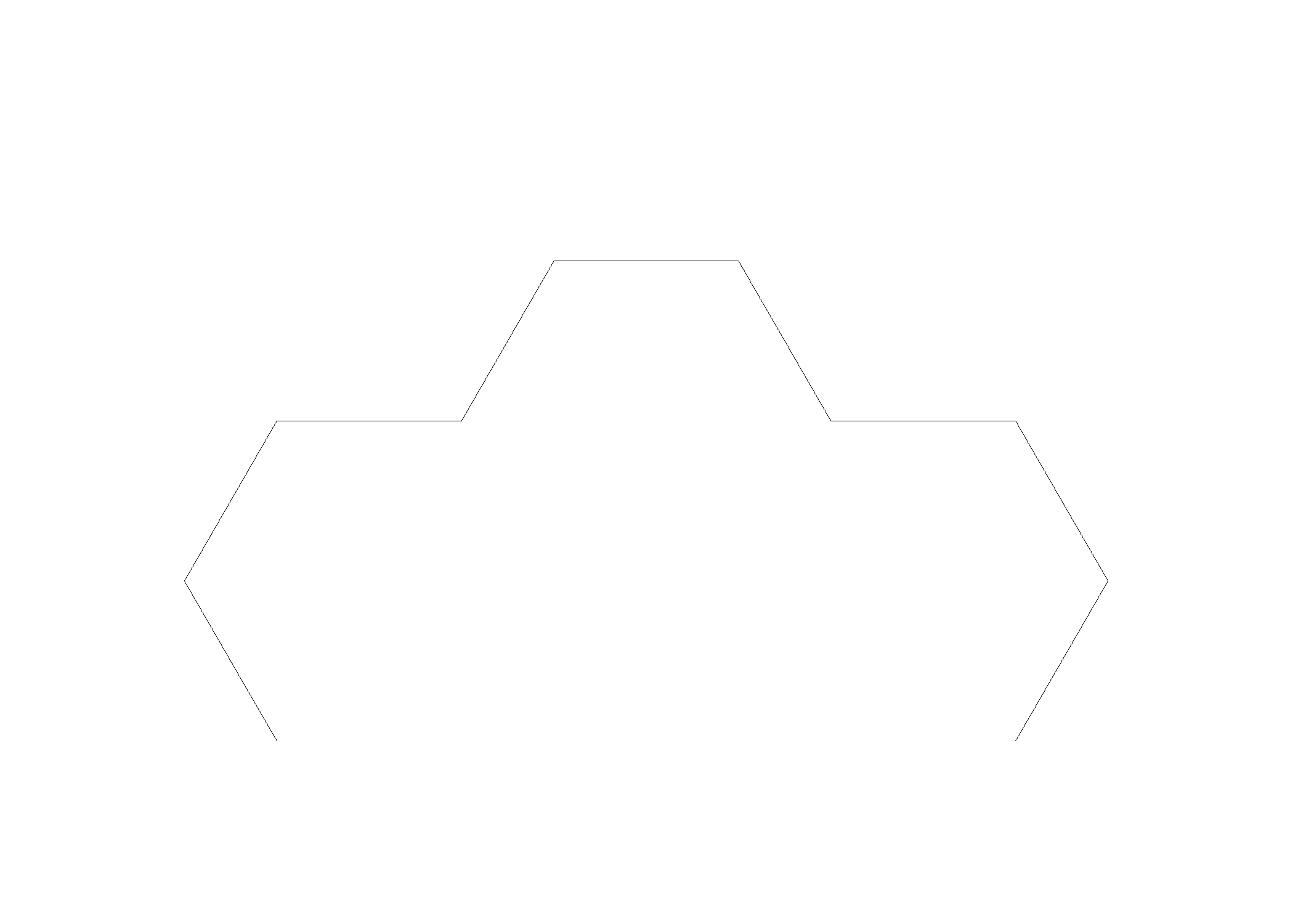
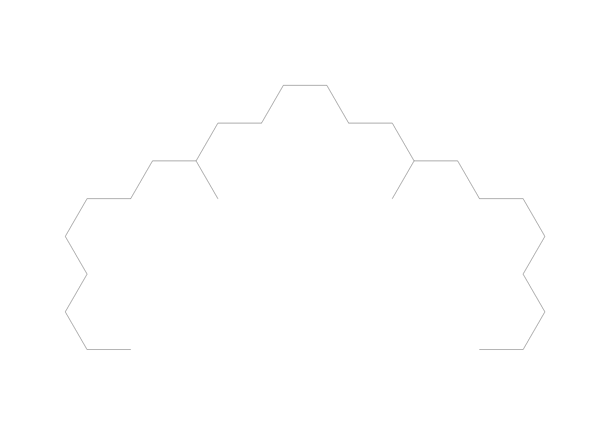
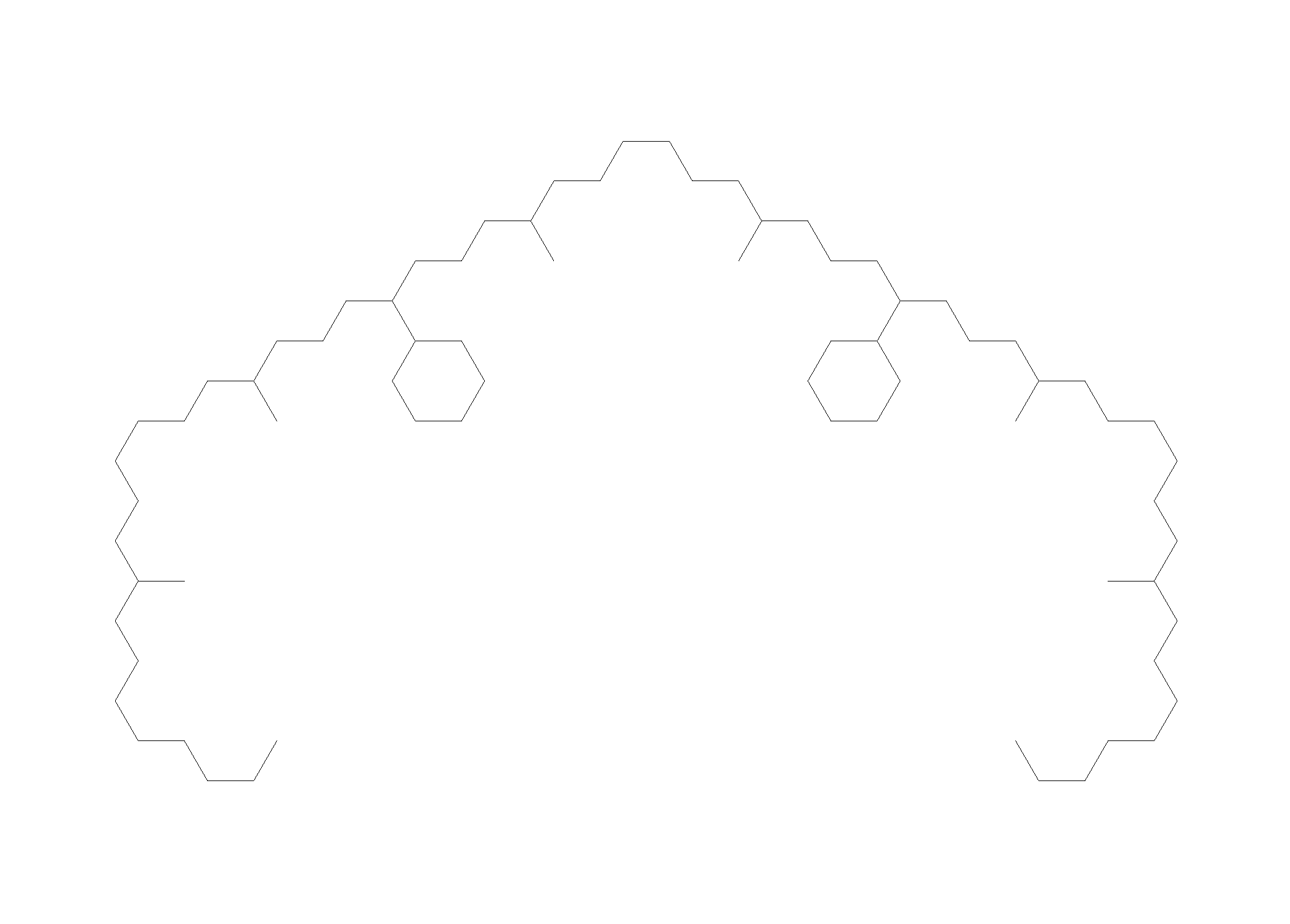
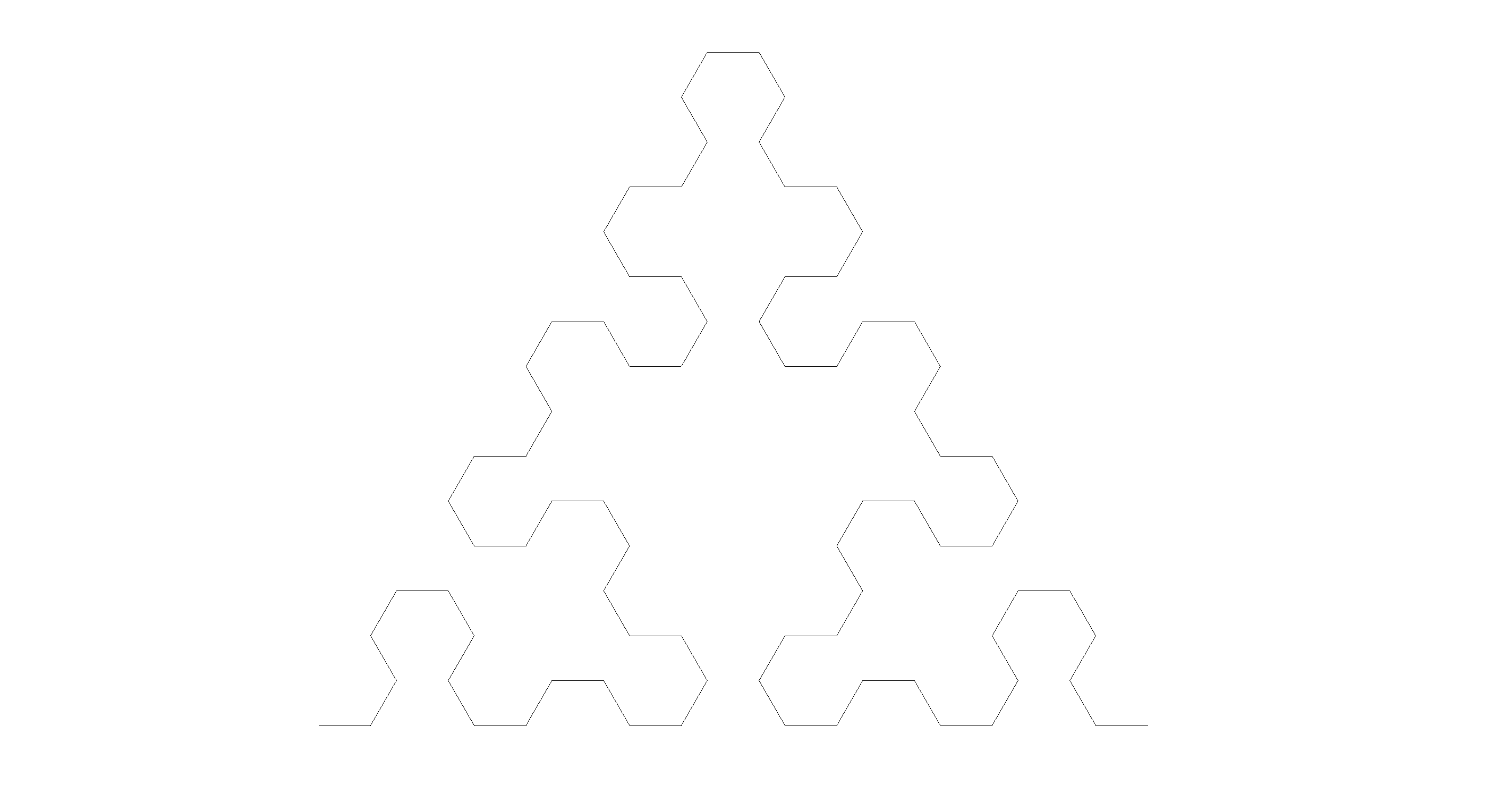
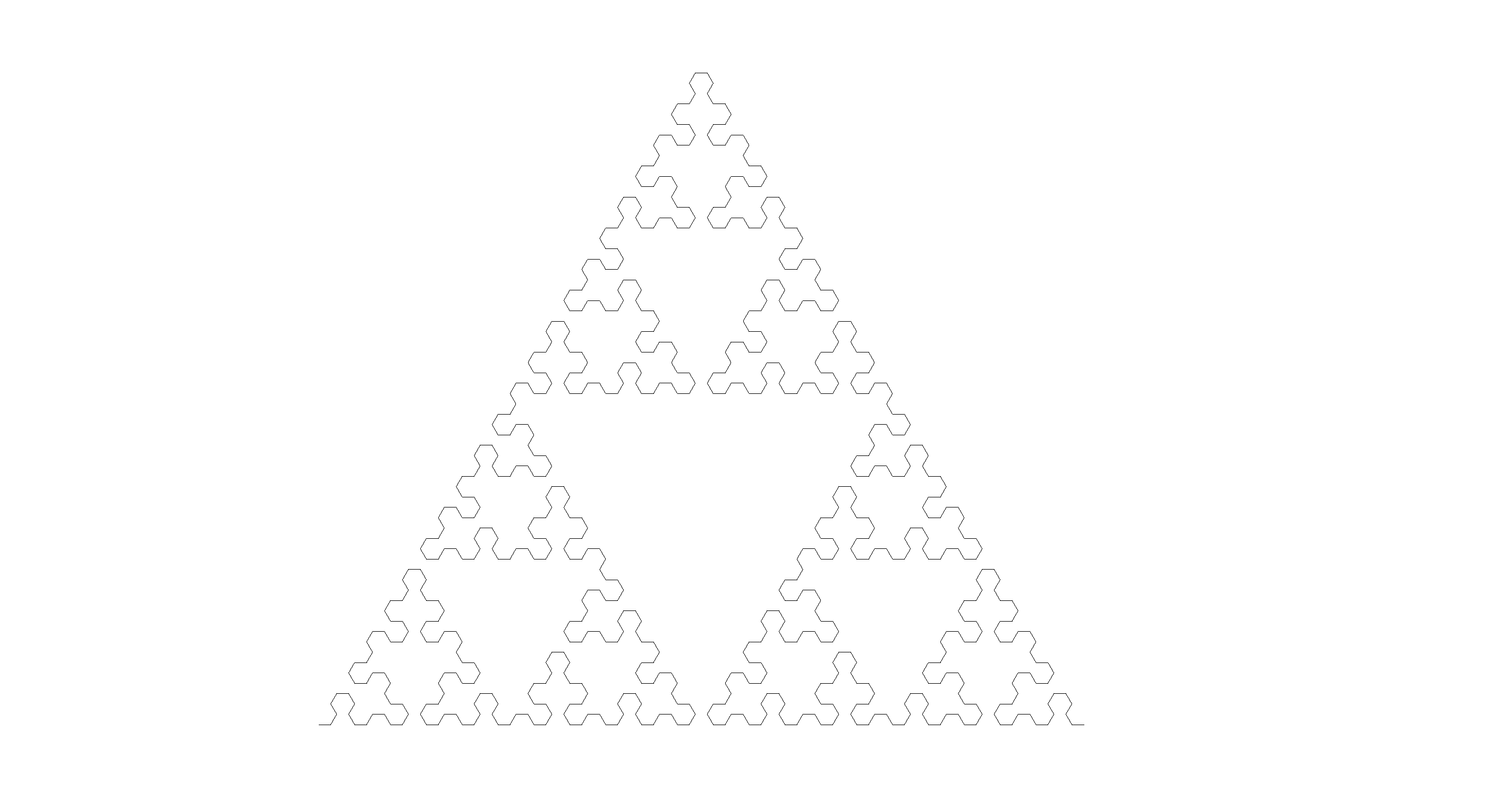
and here is a modifed version of Sierpinski’s triangle that makes fractal snowflakes:

def snowflake_curve(size, recursive_steps):
	if recursive_steps > 0:
		for angle in [60, 60, -60, -60, -60, -60, 60, 60, 0]:
			snowflake_curve(size, recursive_steps-1)
			turtle.left(angle)

	else:
		turtle.forward(size)

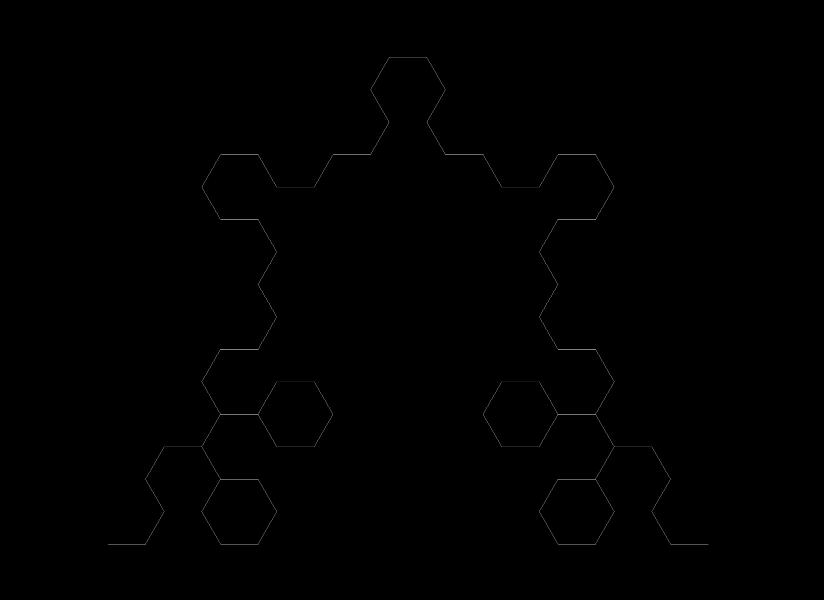
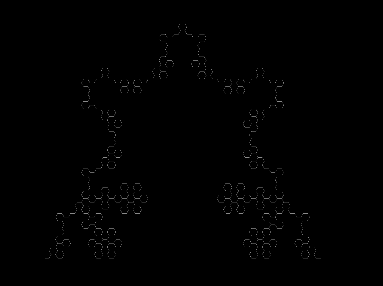
Note that there are smaller snowflakes on the periphery of larger snowflakes: if the recursions were infinite, there would be an infinite number of smaller and smaller snowflakes on these little snowflakes. To save time, the previous image was obtained at a recursive depth of 6.

For more classic fractals and a number of very interesting ideas about fractal geometry in general, see Mandelbrot’s book.

Fractal dimension from box counting

Say one wants to calculate the dimensions of images that are not easily interpreted as self-similar zones as described above. Perhaps the simplest way to do this is to convert the Kolmogorov definition of dimension to a box counting one, which can be proven to have the same limit as the Kolmogorov dimension.

Let’s implement the box counting algorithm. First, importing relevant libraries

# fractal_dimension.py 
# calculates the box counting dimension for thresholded images

from PIL import Image
import numpy as np 
import matplotlib.pyplot as plt
import os

Now for the box counting:

def box_dimension(image_array, min_resolution, max_resolution):
	"""
	Takes an input array (converted from image) of 0s and 
	1s and returns the calculated box counting dimension
	over the range of box size min_resolution (int) to 
	max_resolution (int > min_resolution)
	"""
	assert max_resolution <= min(len(image_array), len(image_array[0])), 'resolution too high'

	counts_array = []
	scale_array = []
	y_size = len(image_array)
	x_size = len(image_array[0])
	for i in range(min_resolution, max_resolution, 5):
		scale_array.append(i)
		count = 0
		for j in range(0, y_size - i, i):
			for k in range(0, x_size - i, i):
				if check_presence(image_array, i, j, k):
					count += 1
		counts_array.append(count)

	# log transform scales and counts
	counts_array = [np.log(i) for i in counts_array]
	scale_array = [np.log(i) for i in scale_array]
	m, b = np.polyfit(scale_array, counts_array, 1) # fit a first degree polynomial

	return m, counts_array, scale_array

which calls the helper function

def check_presence(image_array, i, j, k):
	"""
	Checks for the presence of 1 in a square subarray
	of length i with top left coordinates (j, k).  Returns
	a boolean indicating presence.
	"""
	for x in range(i):
		for y in range(i):
			if image_array[j+y][k+x] == 1:
				return True

	return False

An image must be converted to an array, which forms the input to our program. The following converts an image to an array and thresholds it, in this case for gray pixels on a white background.

path = '/home/bbadger/Desktop/sierpinski/snowflake178.png'

image_array = np.asarray(Image.open(path))
image_ls = []
for i in range(len(image_array)):
	temp = []
	for j in range(len(image_array[i])):
		# thresholding: <130 to find gray pixels
		if any(image_array[i][j] < 130):
			temp.append(1)
		else:
			temp.append(0)
	image_ls.append(temp)

m, counts_array, scale_array = box_dimension(image_ls, 1, 500)
print (f'Fractal dimension: {-m}')

plt.scatter(scale_array, counts_array)
plt.xlabel('log r')
plt.ylabel('log N')
plt.show()
plt.close()

Note that this program is designed for clarity rather than speed, and takes a little over a minute to run for a 1500x2100 image. A faster version may be found here, which reduces this time by a factor of two.

Let’s check this program by using it to calculate the fractal dimension of an object where we can easily find the Hausdorf (scaling) dimension, such as the Sierpinski triangle. For this object, halving the length results in a copy of the original that is 1/3 the ‘volume’, thus this has a Hausdorff dimension of

\[D = \frac{\log N}{\log (1/r)} = \frac{\log 3}{\log 2} \approx 1.585\]

Using box sizes from 1 to 500 pixels, our program yields

which implies a dimension of $d \approx 1.582$, which is close to the true value. For another example, the similarity dimension of the Koch curve is $\log 4 / \log 3 \approx 1.26$, and with box sizes ranging from 1 to 500 pixels our dimensional calculator estimates $d = 1.23$, which is again fairly accurate.

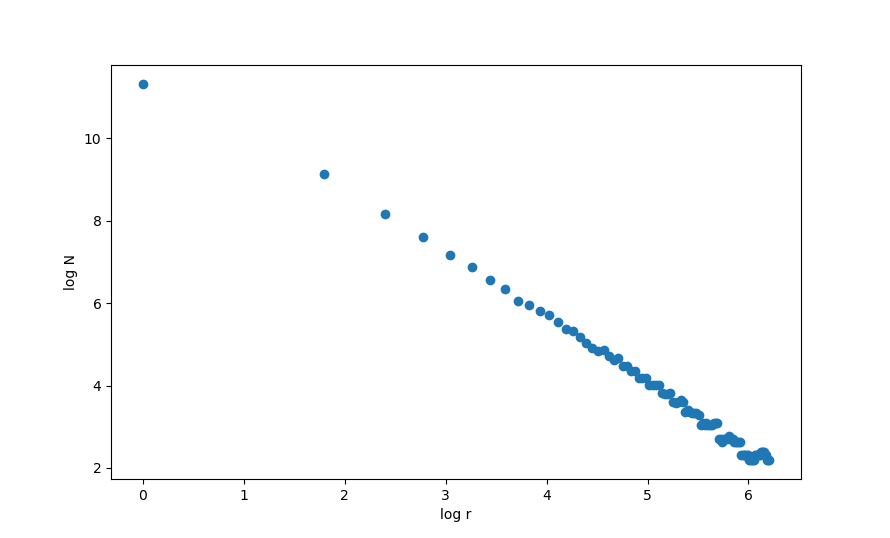
We can also use this program to estimate the dimension of other fractals. The ensuing log/log plot from the snowflake fractal (the last presented in the previous section) is

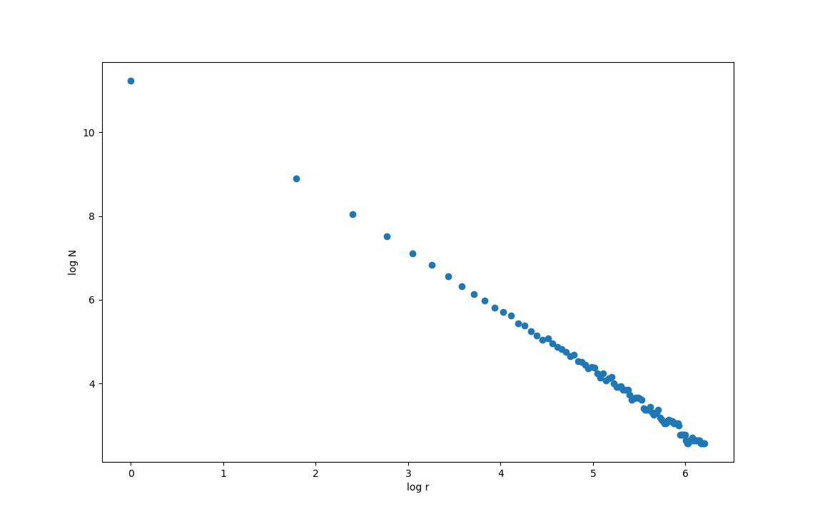
and the dimension is found to be $d \approx 1.45$.

Fractals in the natural world

When I was a kid and just learning how to plot polynomial functions, I remember being quite disappointed to find that any such function describing the objects in the natural world would have to be extremely complicated and unwieldy. Nearly every shape in nature, from the outline of the trees around my parent’s house to the pattern or surf on the seaside to the shapes of nebulae and galaxies I saw in astronomy books were all, as I found, unsuitable for attempting to recreate using the functions I knew then (polynomial and trigonometric functions).

I did not know at the time, but there is a good reason from this. These shapes are non-differentiable: increasing in scale does not lead to a simpler, more line-like shape. Rather, one finds more detail the closer one looks. These shapes are better mathematically described using fractal geometry, and why this is should be evident from the fractals that have been drawn above. Fractals also contain more detail the closer one looks, and thus are non-differentiable. Simple rules specify intricate shapes.

Fractals can be thought of as shapes that are irregular and do not become more regular as one increases scale, as well as shapes that have smaller parts that resemble the whole. TA particularly noteworthy example of both of these properties exists in coastlines. Here is a picture of the Chesapeake Bay taken from a satellite which is found in the Smithsonian museum.

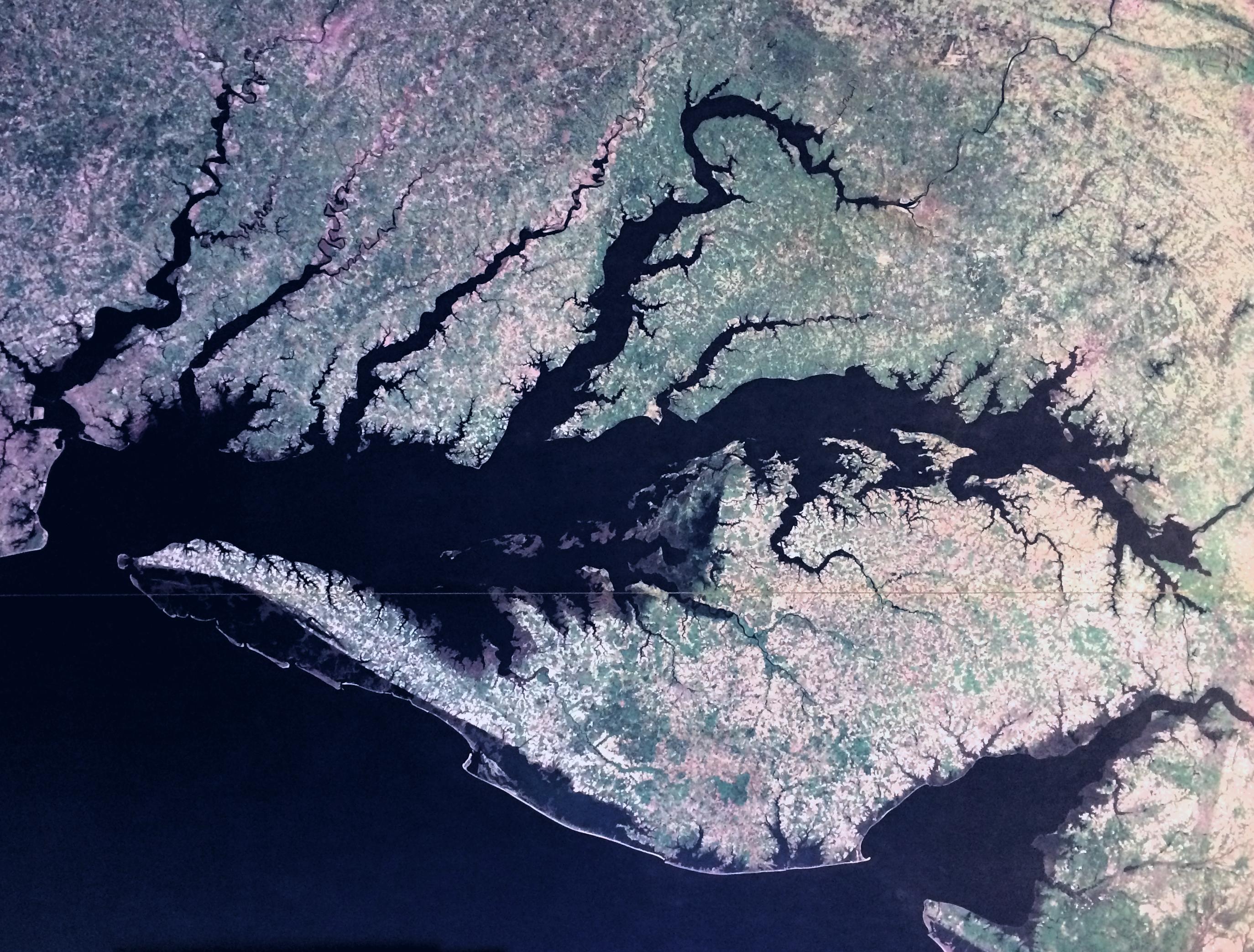
Observe how the large bay has many smaller bays that, though not identical in shape, closely resemble the whole bay. These inlets in turn have smaller inlets and so on past the resolution limit of this image. This makes the coastline irregular on a large scale but importantly that this irregularity does not diminish with an increase in scale.

The length of the coastline in the image above is entirely dependent on how high the resolution of the image is: a higher resolution image will yield a larger measurement. This is not the case for smooth objects that we like to measure, such as the desk I am writing on. In addition, fractals are non-differentiable: calculus cannot be accurately applied to these objects because at many points they do not have a defined tangent curve.

What does this matter, beyond the purpose of attempting to model nature in the most parsimonious fashion? The observation that most objects in the natural world are best described as fractals is important because it implies that nearly all natural dynamical processes are nonlinear. Being that the vast (vast) majority of all possible mathematical functions are nonlinear, it may come as little surprise that most things that change over time in the natural world are best described using nonlinear functions. But consider what this means for scientific inquiry, both past and present. Linear mathematical transformations are scaling and additive: they can be decomposed into parts and then reassembled. Nonlinear transformations are not additive and therefore cannot be analyzed by decomposition into parts.

Linearity is often assumed when experimental scientific models are constructed and tested. For an example, first consider the Schrodinger equation which forms the basis of the wave equations of quantum mechanics. This equation is linear, and if it were not then the principle of superposition would not be applicable.

The fractal geometries seen at many scales in nature suggest that linear models are generally not accurate, as only nonlinear dynamical systems can exhibit fractal attractors. And in observational scientific disciplines such as general relativity, for example, models are often based on nonlinear differential equations. But there is something important to remember about such equations: they are unsolvable except under special circumstances. This means that we can predict how celestial bodies may curve spacetime, but these predictions are necessarily imperfect.