The Henon map
Michel Hénon sought to recapitulate the geometry of the Lorenz attractor in two dimensions. This requires stretching and folding of space, achieved with the following discrete system, which is now referred to as the Henon map:
\[x_{n+1} = 1-ax_n^2 + y_n \\ y_{n+1} = bx_n \tag{1} \label{eq1}\]When
\[a = 1.4 \\ b = 0.3 \\ x_0, y_0 = 0, 0\]the result may be plotted using python as follows:
#python3
import numpy as np
import matplotlib.pyplot as plt
plt.style.use('dark_background')

def henon_attractor(x, y, a=1.4, b=0.3):
	'''Computes the next step in the Henon
	map for arguments x, y with kwargs a and
	b as constants.
	'''
	x_next = 1 - a * x ** 2 + y
	y_next = b * x
	return x_next, y_next

# number of iterations and array initialization
steps = 100000
X = np.zeros(steps + 1)
Y = np.zeros(steps + 1)

# starting point
X[0], Y[0] = 0, 0

# add points to array
for i in range(steps):
	x_next, y_next = henon_attractor(X[i], Y[i])
	X[i+1] = x_next
	Y[i+1] = y_next

# plot figure
plt.plot(X, Y, '^', color='white', alpha = 0.8, markersize=0.3)
plt.axis('off')
plt.show()
plt.close()
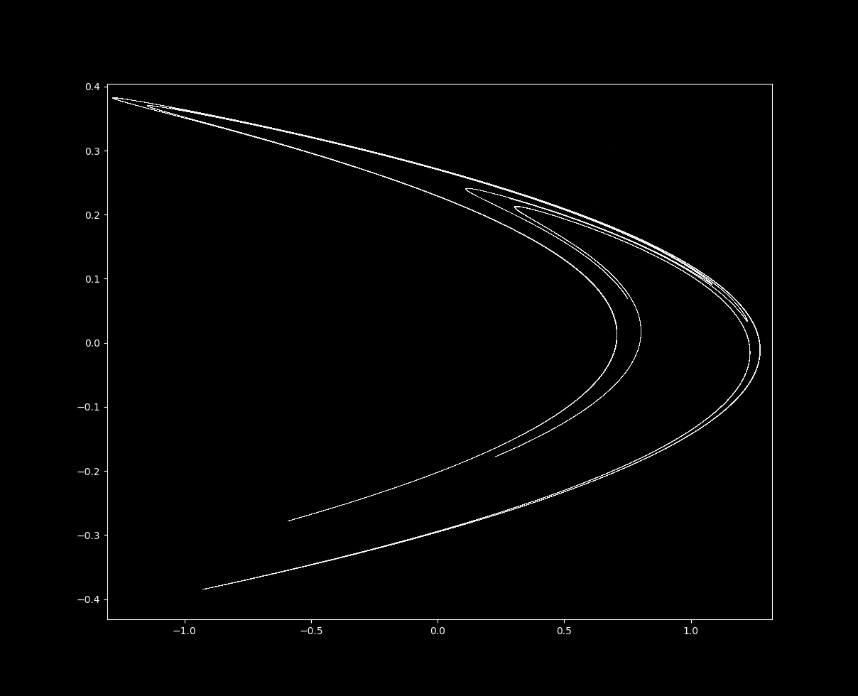
After many iterations, the following map is produced:
How does the equation produce the map above? We can plot each point one by one to find out. To do this, the program above can be modified as follows to make many images of the map of successive iterations of \eqref{eq1}, which can then be compiled into a movie (see here for an explanation on how to compile images using ffmpeg).
...

for i in range(steps):
	x_dot, y_dot = henon_attractor(X[i], Y[i])
	X[i+1] = x_dot
	Y[i+1] = y_dot
	plt.xlim(-1.5, 1.5)
	plt.ylim(-0.5, 0.5)

	plt.plot(X, Y, '^', color='white', alpha = 0.8, markersize=0.3)
	plt.axis('off')
	plt.savefig('{}.png'.format(i), dpi=300)
	plt.close()
For the first thousand iterations:
Successive iterations jump around unpredictably but are attracted to a distinctive curved shape.
The Henon map is a strange (fractal) attractor
For certain starting values $x_0, y_0$, \eqref{eq1} with a=1.4 and b=0.3 does not head towards infinity but is instead attracted to the region shown above. This shape is called an attractor because regardless of where $x_0, y_0$ is placed, if subsequent iterations do not diverge then they are drawn to the shape above.
Let’s examine this attractor. If we increase magnification on the top line in the center, we find that it is not a line at all! With successive increases in magnification (and more iterations of \eqref{eq1}), we can see that each top line is actually many lines close together, in a self-similar pattern. This is indicative of a fractal shape called the Cantor set.
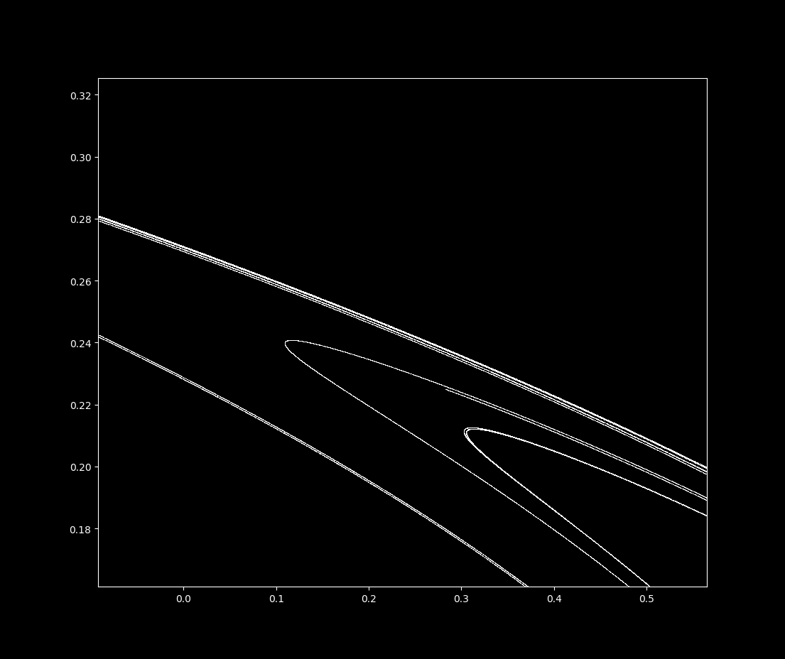
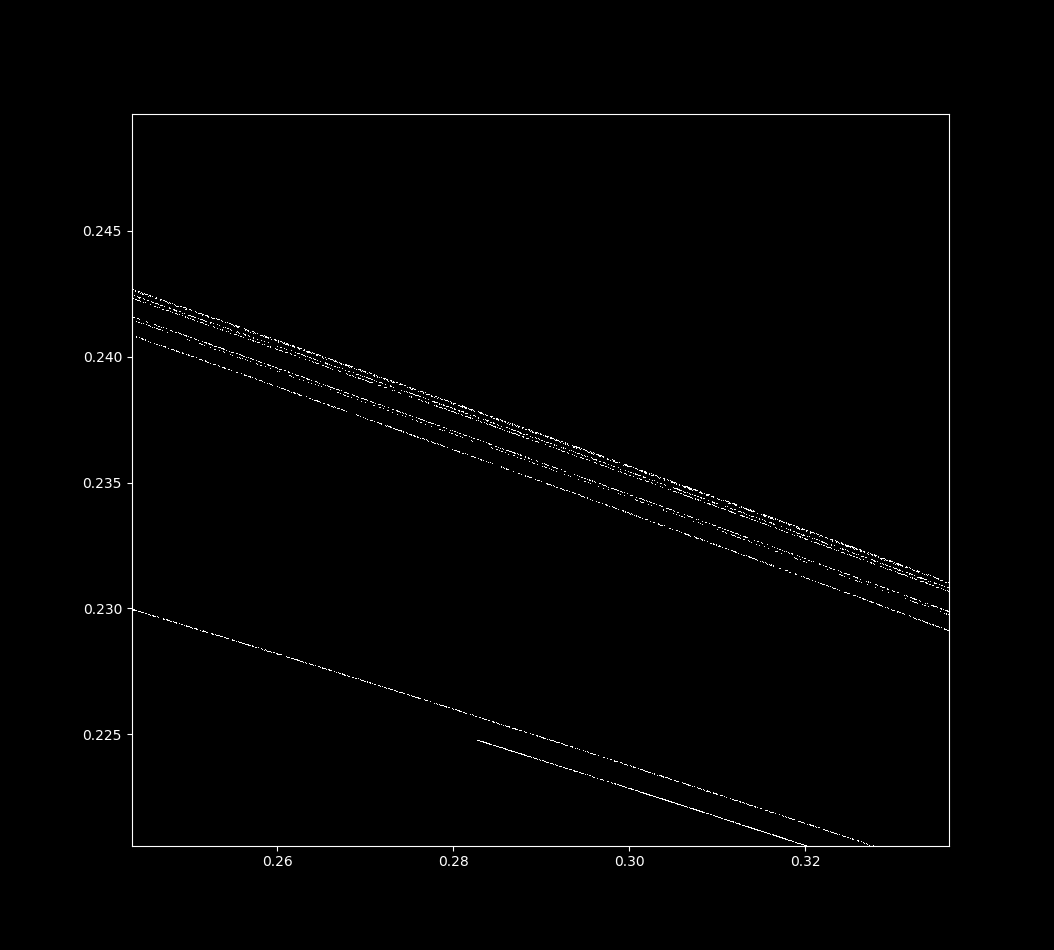
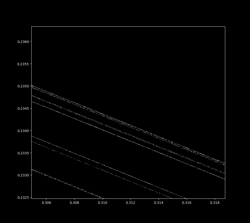
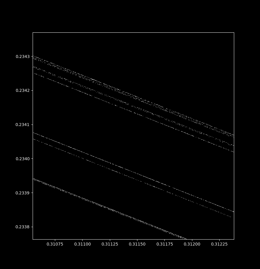
In general terms, the Henon map is a fractal because it looks similar at widely different scales. Zooming in near the point (x, y) = (0.3114164… , 0.234185….), we have
The boundary of the basin of attraction for the Henon map
Some experimentation can convince us that not all starting points head towards the attractor upon successive iterations of \eqref{eq1} with $a=1.4$ and $b=0.3$: instead, some head towards positive or negative infinity! The collection of points that do not diverge (head towards infinity) for a given dynamical system is called the basin of attraction. Basins of attraction may be fractal or else smooth as shown by Yorke. Does the Henon map (with $a=1.4, b=0.3$) have a smooth or fractal basin?
To find out, let’s import the necessary libraires and define a function henon_boundary as follows
#! python3
# import third-party libraries
import numpy as np
import matplotlib.pyplot as plt
plt.style.use('dark_background')
import copy

def henon_boundary(max_iterations, a, b):
	''' A function to show the basin of attraction for
	the Henon map.  Takes in the desired number of maximum
	iterations and the a and b values for the Henon equation,
	returns an array of the number of iterations until divergence
	'''
Now we can initialize the size of the image (in pixels) we want to make by specifying values for variables x_range and y_range. A list of points for each variable is made over this range, and x- and y- arrays (array[0] and array[1]) are formed using the np.meshgrid class. This array will store the values of each point as \eqref{eq1} is iterated. Next we need an array to store the number of iterations until divergence, which can be accomplished (not particularly efficiently) by making an array of 0s in the same shape as the array and then adding the maximum iteration number to each array element.
	x_range = 2000
	y_range = 2000

	x_list = np.arange(-5, 5, 10/x_range)
	y_list = np.arange(5, -5, -10/y_range)
	array = np.meshgrid(x_list, y_list)

	x2 = np.zeros(x_range)
	y2 = np.zeros(y_range)
	iterations_until_divergence = np.meshgrid(x2, y2)

	for i in iterations_until_divergence:
		for j in i:
			j += max_iterations
In an effort to prevent explosion of values to infinity, we will run into the possibility that some values can diverge more than once. To prevent this, we can make a boolean array not_alread_diverged in which every element is set to True (because nothing has diverged yet).
	# make an array with all elements set to 'True'
	not_already_diverged = array[0] < 1000
Now we iterate over the array to find when each position diverges towards infinity (if it does). Because iteration of \eqref{eq1} is a two-step process, the x-array is copied such that it is not modified before being used to make the new y-array. A boolean array diverging is made, signifying whether or not the distance of any point has become farther than 10 units from the origin, which I use as a proxy for divergence. By using bitwise and, we make a new array diverging_now that checks whether divergence has already happened or not, and assigns True only to the diverging values that have not. The indicies of iterations_until_divergence that are currently diverging are assigned to the iteration number k, and the not_already_diverged array is updated. Finally, diverging elements of x or y arrays are then assigned as 0 to prevent them from exploding to infinity (as long as the origin does not head towards infinity, that is).
	for k in range(max_iterations):
		array_copied = copy.deepcopy(array[0]) # copy array to prevent premature modification of x array

		# henon map applied to array
		array[0] = 1 - a * array[0]**2 + array[1]
		array[1] = b * array_copied

		# note which array elements are diverging but have not already diverged
		r = (array[0]**2 + array[1]**2)**0.5
		diverging = r > 10
		diverging_now = diverging & not_already_diverged
		iterations_until_divergence[0][diverging_now] = k
		not_already_diverged = np.invert(diverging_now) & not_already_diverged

		# prevent explosion to infinity
		array[0][diverging] = 0
		array[1][diverging] = 0

	return iterations_until_divergence[0]
And now this may be plotted. To overlay the henon map with the attractor basin, the basin map must be scaled appropriately using the kwarg extent.
plt.plot(X, Y, ',', color='white', alpha = 0.8, markersize=0.3)
plt.imshow(henon_boundary(70, a=0.2, b=-0.909 - t/6000), extent=[-5, 5, -5, 5], cmap='twilight_shifted', alpha=1)
plt.axis('off')
plt.savefig(Henon_boundary.png', dpi=300)
plt.close()
Let’s see what happens to the basin of attraction and the attractor itself when $a$ is increased from $1$ to $1.48$ (constant $b=0.3$):
The attractor is visible as long as it remains in the basin of attraction. This intuitively makes sense: there is nothing special about the original points compared to subsequent iterations. If points in an attractor were drawn to a region that then blew up to infinity, the attractor would be no more no matter where the starting point was located. Focusing on the transition from smooth to fractal form in the basin of attraction, we can see this coincides with the disappearence of the attractor itself:
This abrupt change between smooth and fractal attractor basin shape is called basin metamorphosis.
A semicontinuous iteration of the Henon map reveals period doubling
This map \eqref{eq1} is discrete, but may be iterated using Euler’s method as if we wanted to approximate a continuous equation:
\[\cfrac{dx}{dt} = 1-ax^2 + y \\ \cfrac{dy}{dt} = bx_n \\ x_{n+1} \approx x_n + \cfrac{dx}{dt} \cdot \Delta t \\ y_{n+1} \approx y_n + \cfrac{dy}{dt} \cdot \Delta t \\ \tag{3}\]With larger-than-accurate values of $\Delta t$, we have a not-quite-continuous map that can be made as follows:
# import third-party libraries
import numpy as np
import matplotlib.pyplot as plt
plt.style.use('dark_background')

def henon_attractor(x, y, a=.1, b=0.03):
	'''Computes the next step in the Henon
	map for arguments x, y with kwargs a and
	b as constants.
	'''
	dx = 1 - a * x ** 2 + y
	dy = b * x
	return dx, dy

# number of iterations and step size
steps = 5000000
delta_t = 0.0047

X = np.zeros(steps + 1)
Y = np.zeros(steps + 1)

# starting point
X[0], Y[0] = 1, 1

# compute using Euler's formula
for i in range(steps):
	x_dot, y_dot = henon_attractor(X[i], Y[i])
	X[i+1] = X[i] + x_dot * delta_t
	Y[i+1] = Y[i] + y_dot * delta_t

# display plot
plt.plot(X, Y, ',', color='white', alpha = 0.1, markersize=0.1)
plt.axis('on')
plt.show()
If iterate (3) with $a=0.1, b = 0.03, \Delta t = 0.047 $, the following map is produced:
It looks like the orbit plot for the logistic map! As this system is being iterated semicontinuously, we can observe the vectorfield that the motion of the points:
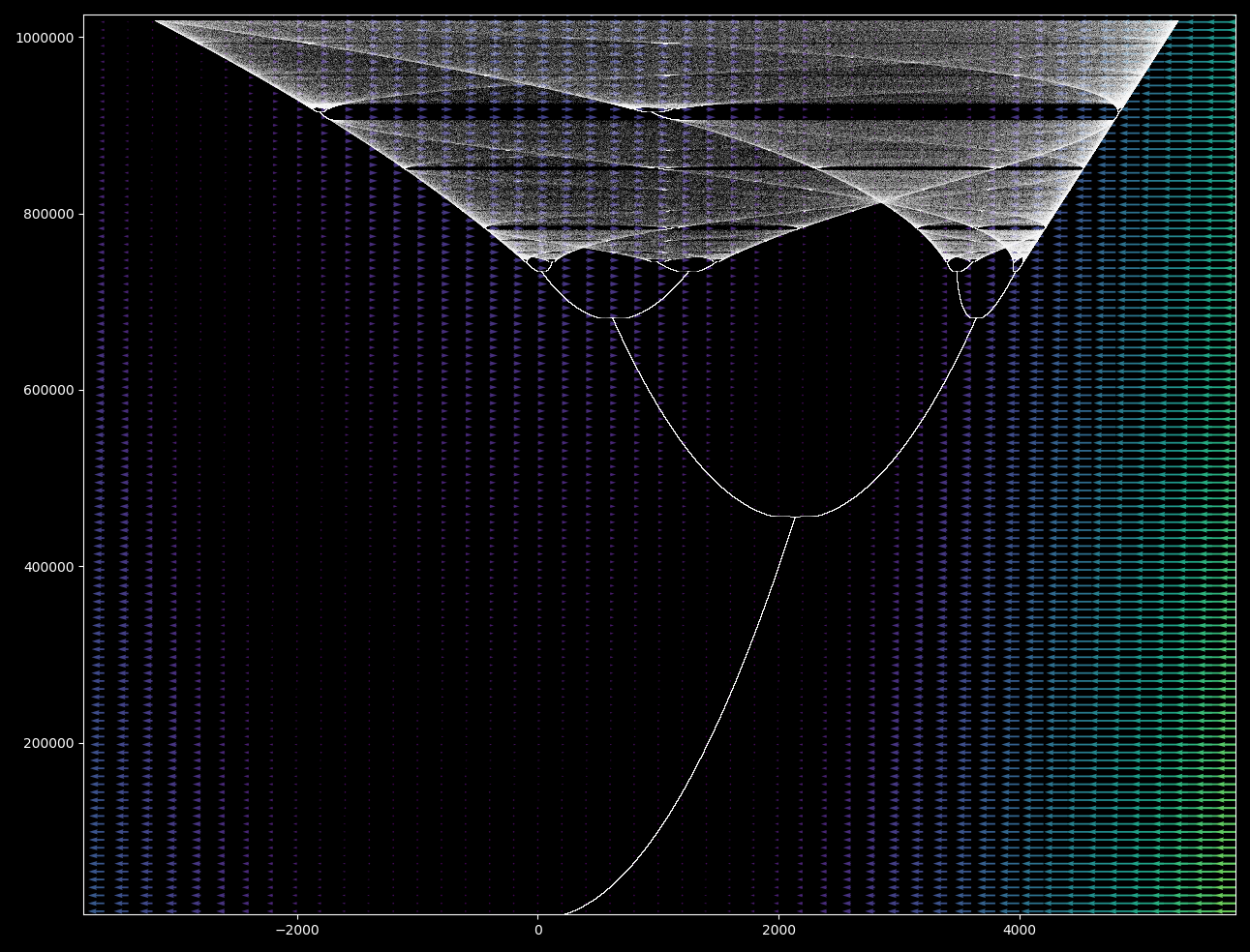
Subsequent iterations after the first bifurcation lead to the point bouncing from left portion to right portion in a stable period. In the region of chaotic motion of the point, the vectors are ordered.
Why is this? The Henon map has one nonlinearity: an $x^2$. Nonlinear maps may transition from order (with finite periodicity) to chaos (a period of infinity for most points) with changes in parameter values. The transition from order to chaos for many systems occurs via period doubling leading to infinite periodicity in finite time, resulting in a logistic-like map.
Renaming $\Delta t$ to $d$ for clarity, we have
\[x_{n+1} = x_n + (1-ax_n^2 + y) \Delta t \\ x_{n+1} = x_n + d - adx_n^2 + dy \\ x_{n+1} = -adx_n^2 + x_n + d(1+y)\]Notice the similarity to the quadratic equation
\[x_{n+1} = x_n^2 + c\]If an orbit map of the quadratic equation (see this page for explanation) where the horizontal axis corresponds to $x_n$ iterations and the vertical axis to $c$ values, multiplied by negative 1 (the actual range is 0 to -2):
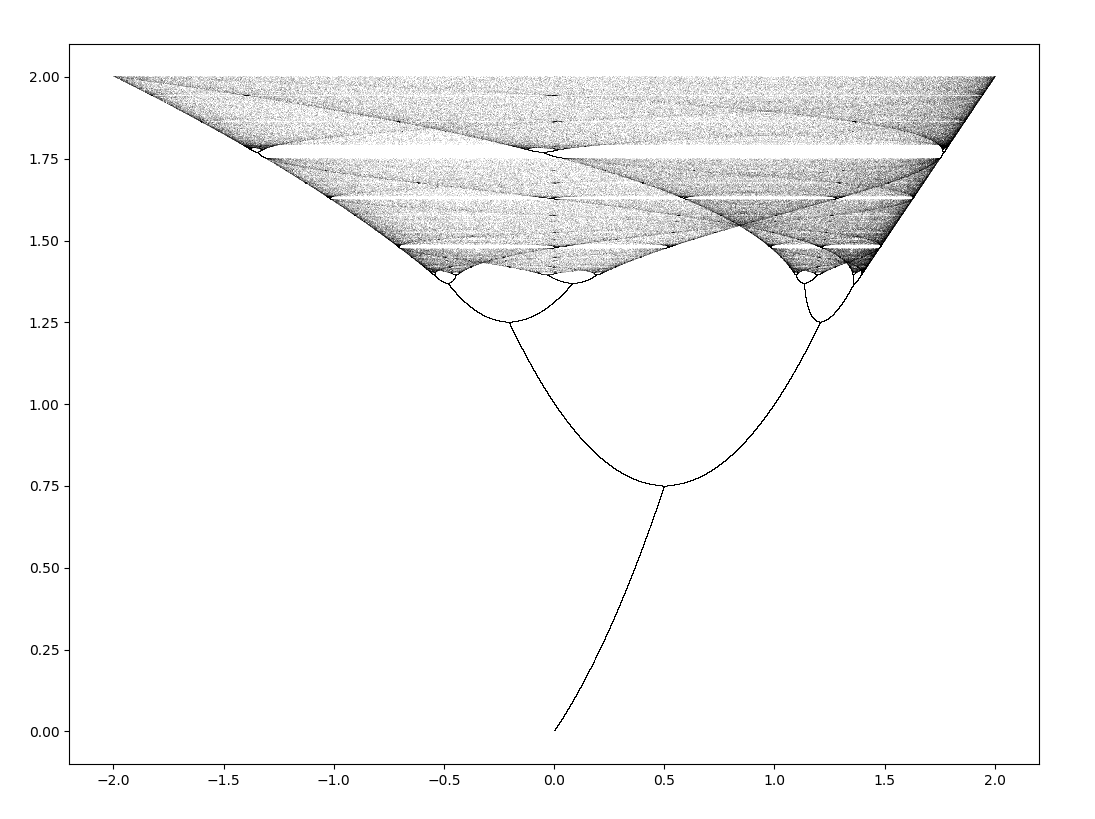
The orbit map for the quadratic equation displays the same periodicity to aperiodicity pattern as the logistic map with period doubling and a chaotic region. It looks nearly identical to this semicontinuous Henon orbit map! Could these orbits actually be the same, only in different notation?
Given the two equations
\[f(x) = x^2 + c \\ g(x) = -adx^2 + x + d + dy\]and a linear transformation,
\[h(x) = mx + b\]and being that linear transformations do not change the topological properties of a set (they are homeomorphic transformations), if it can be shown that
\[h^{-1} \circ f \circ h = g\]or equivalently that
\[h^{-1}(f(h(x))) = g(x) \\ f(h(x)) = h(g(x))\]then $f(x)$ is dynamically equivalent to $g(x)$ because these are topological conjugates of one another.
Expanding these expressions and simplifying, we have
\[(mx+b)^2 + c = m^2x^2 + 2mbx + b^2 + c \\ m(-adx^2 + x + d + dy) + b \implies \\ mx^2+2bx + \frac{b^2}{m} + \frac{c}{m} = -adx^2 + x + d + dy + \frac{b}{m}\]now by a change of variables,
\[m = -ad \implies 2bx + \frac{b^2}{-ad} + \frac{c}{-ad} = x + d + dy + \frac{b}{-ad} \\ b = 1/2 \implies \frac{c}{-ad} = d + dy + \frac{1}{-4ad} \\\]and therefore
\[c = -ad \left( d+dy-\frac{1}{4ad} \right) = -ad^2(1+y) + 1/4\]results in $f(h(x)) = h(g(x))$, which can be checked by substituting the values obtained for $m, \; b, \; c$ and simplifying. This being the case, these two expressions are conjugates of each other, meaning that it is no surprise that they are capable of displaying nearly identical dynamics.
Pendulum map from the Henon attractor
This is not the only similarity the Henon map has to another dynamical system: \eqref{eq1} can also result in a map that displays the waves of the semicontinuous pendulum map. The $a, b$ values yielding the spiral patterns were found here.
Setting $a=0.2, b=-0.99994$ and $x_0, y_0 = -1.5, 1.5$ we have
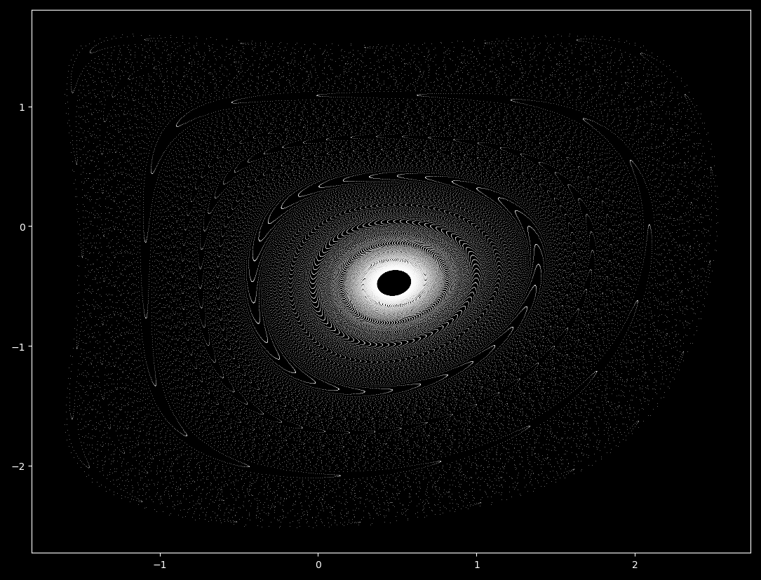
The semicontinuous pendulum waves form as a spiral trajectory unwinds with increasing $\Delta t$. Does this Henon map form the same way? Let’s find out by plotting \eqref{eq1} going from $b \approx -0.9 \to b \approx -1.05$, including the attractor basin.
Similarly, at $a=0.2, b=0.999448$ and $x_0, y_0 = 0, 0$, there are two pendulum-like maps
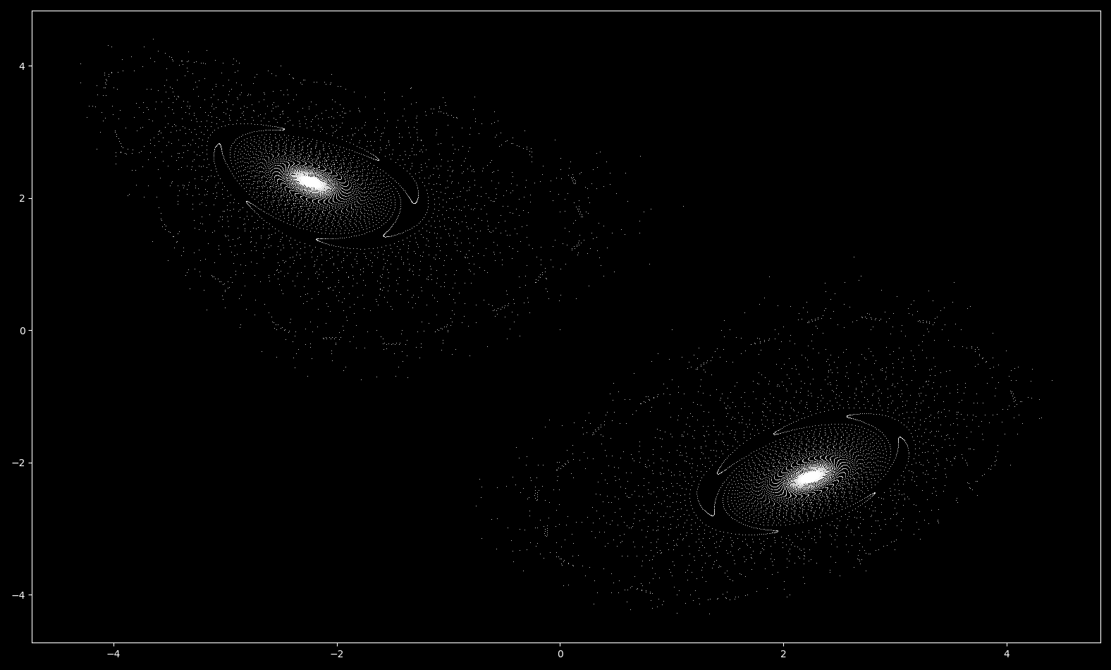
which form as spirals unwind before the attractor basin collapses from $b=0.95 \to b\approx 1.05$:
Thus the waves of the henon map form in a similar fashion to those seen in the pendulum phase space. But there is a significant difference between these two maps: the Henon spiral does not settle on a periodic orbit (as is the case for the pendulum map for certain parameter values) but continues to head towards a point attractor as long as 0 > b > -1.
Note that unlike the case for $a=1.4, b=0.3$, the basin of attraction is a fractal while a stable attractor remains. The fractal edge of the basin of attraction extends outward when the attractor remains (as for the spiral maps) but extends inward into the attractor space in the region of $a=1.4, b=0.3$.
To observe the behavior of stable and unstable points for the Henon map iterated in reverse, see this page.
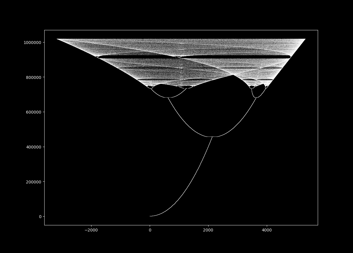
Fractal zoom on a henon map divergence
At $a=0.2$ and $b=-1.1$, points head towards infinity nearly everywhere. One point that does not diverge is where the next iteration is equivalent to the current, or where $x_{n+1} = x_n$ and $y_{n+1} = y_n$. This can be found as follows:
\[x_n = 1 - ax_n^2 + y_n \\ y_n = bx_n \implies \\ 0 = 1-ax_n^2 + (b-1)x_n + 1 \\\]which by the quadratic formula yields
\[x_n = \frac{(b-1) \pm \sqrt{(b-1)^2 + 4a}}{2a} \\ y_n = bx_n\]When $a = 0.2, b = -1.1$ is substituted into this equation system, we can evaluate two non-diverging points at $(x, y) \approx (0.456, -0.502)$ and $(x, y) \approx (-10.956, 12.052)$. Both coordinates are unstable: only the (irrational) values of
\[x = \frac{(-2.1) \pm \sqrt{(-2.1)^2 + 0.8}}{0.4} \\ y = -1.1x\]will remain in place for an arbitrary number of iterations. Approximations, no matter how accurate, will diverge over time. This is important because there are no perfect finite representations of irrational numbers, meaning that any form of the radical above that can be stored in finite memory will eventually diverge to infinity given enough iterations of \eqref{eq1}.
The former coordinate lies at the center of the pinwheel, meaning that regions nearby converge more slowly than regions elsewhere and is therefore semistable. The latter point is unstable, such that iterations arbitrarily close rapidly diverge. To get an idea of just how unstable this point is, for $(x, y) \approx (-10.956, 12.052)$ at 64 bit precision (meaning that x is defined as -10.956356105256663), divergence occurs after a mere ~28 iterations. In contrast, it takes over five hundred iterations for $(x, y) \approx (0.456, -0.502)$ at 64 bit precision to diverge.
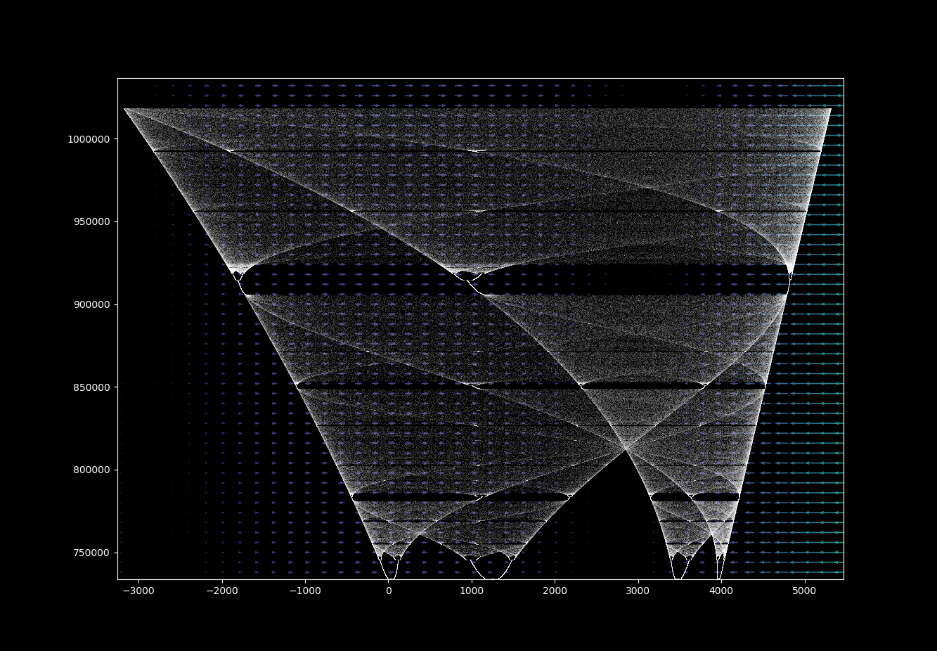
Let’s zoom in on the pinwheel-like pattern of slower divergence around $(x, y) \approx (0.456, -0.502)$ to get an appreciation of its structure! The first step is to pick a point and then adjust the array the graph is produced on accordingly.
def henon_map(max_iterations, a, b, x_range, y_range):
	# offset slightly from true value
	xl = -5/(2**(t/15)) + 0.4564
	xr = 5/(2**(t/15)) + 0.4564
	yl = 5/(2**(t/15)) - 0.50202
	yr = -5/(2**(t/15)) - 0.50202

	x_list = np.arange(xl, xr, (xr - xl)/x_range)
	y_list = np.arange(yl, yr, -(yl - yr)/y_range)
	array = np.meshgrid(x_list, y_list)
Now we can plot the images produced (adjusting the extent variable if the correct scale labels are desired) in a for loop. I ran into a difficulty here that I could not completely debug: the diverging array in the henon_map() function occasionally experienced an off-by-one error in indexing: if the array[0] dimensions are 2000x2000, the diverging array would become 2001x2001 or 2002x2002 etc. The root of this problem is a round off error in the array size calculation (here 10 / x_range). Although the workaround above is effective, the simplest and most efficient way of addressing this is to simply take the correct number of indicies of the x_list and y_list arrays when making the two dimensional array.
...
def henon_boundary(max_iterations, a, b):
	x_range = 2000
	y_range = 2000

	x_list = np.arange(-5, 5, 10/x_range)
	y_list = np.arange(5, -5, -10/y_range)
	array = np.meshgrid(x_list[:2000], y_list[:2000])
...
When $a=0.2, b=-1.1$, increasing the scale by a factor of $2^{20}$ around the point $(x, y) = (0.4564, -0.50202)$, we have