Periodicity and reversibility
Suppose one were to observe movement over time, and wanted to describe the movement mathematically in order to be able to predict what happens in the future. This is the goal of dynamical theory, and other pages on this site should convince one that precise knowledge of the future is much more difficult than it would seem even when a precise dynamical equation is known.
What about if someone were curious about the past? Given a system of dynamical equations describing how an object’s movement occurs, can we find out where the object came from? This question is addressed here for two relatively simple iterative systems, the logistic and Henon maps.
The logistic map is non-invertible
The logistic equation, which has been explored here and here is as follows:
\[x_{n+1} = rx_n(1-x_n) \tag{1} \label{eq1}\]The logistic equation is a one-dimensional discrete dynamical map of very interesting behavior: periodicity for some values of $r$, aperiodicity for others, and for $0 < r < 4$, the interval $(0, 1)$ is mapped into itself.
What does \eqref{eq1} look like in reverse, or in other words given any value $x_{n+1}$ which are the values of $x_n$ which when evaluated with \eqref{eq1} yield $x_{n+1}$? Upon substituting $x_n$ for $x_{n+1}$,
\[x_n = rx_{n+1}(1-x_{n+1}) \\ 0 = -rx_{n+1}^2 + rx_{n+1} - x_n \\\]The term $x_n$ can be treated as a constant (as it is constant for any given input value $x_n$), and therefore we can solve this expression for $x_{n+1}$ with the quadratic formula $ax^2 + bx + c$ where $a = -r$, $b = r$, and $c = -x_n$, to give
\[x_{n+1} = \frac{r \pm \sqrt{r^2-4rx_n}}{2r} \tag{2} \label{eq2}\]Now the first thing to note is that this dynamical equation is not strictly a function: it maps a single input $x_n$ to two outputs $x_{n+1}$ (one value for $+$ or $-$ taken in the numerator) for many values of $x_n \in (0, 1)$ whereas a function by definition has one output for any input that exists in the pre-image set. In other words the logistic map is non-invertible.
The aperiodic logistic map in reverse is unstable
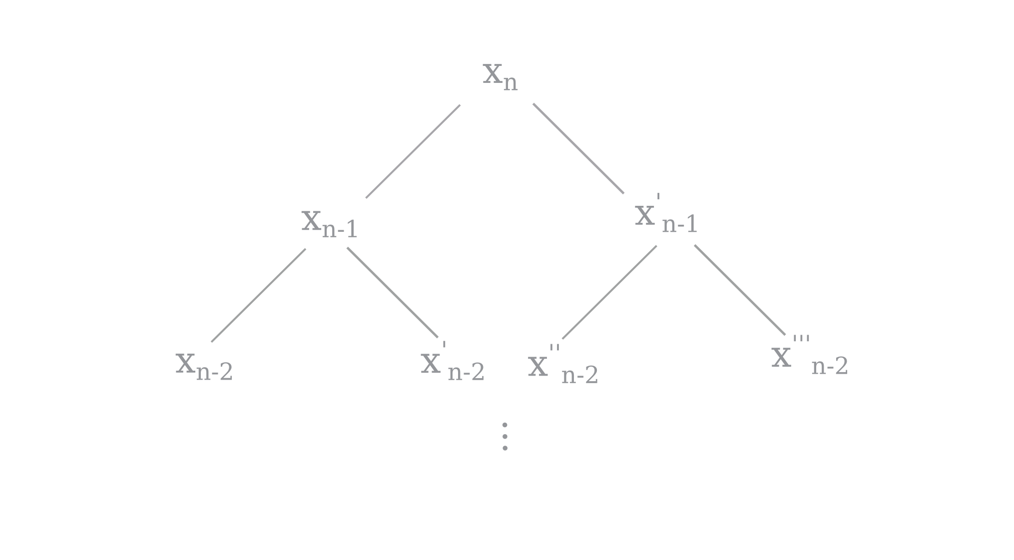
What does it mean for a dynamical equation to be non-invertible? It means that, given a point in a trajectory, we cannot determine what its previous point was with certainty. In the case of the reverse logistic equation \eqref{eq2}, one point $x_n$ could have two possible previous points $x_{n-1}, x_{n-1}’$ and each of these could have two possible previous points $x_{n-2}, x_{n-2}’, x_{n-2}’’, x_{n-2}’’’$ and so on (note that some points have only one previous point, because either $x_{n-1}, x_{n-1}’ \not \in (0, 1)$).
Suppose one wanted to calculate the all the possible values that could have preceded $x_n$ after a certain number of steps. The set s of points a point could have come from after a given number of steps may be found using recursion on \eqref{eq2} as shown below:
def reverse_logistic_map(r, array, steps, s):
	# returns a set s of all possible values of
	# the reverse logistic starting from array[0]
	# after a given number of steps
	if steps == 0:
		for i in array:
			s.add(i)
		return

	array_2 = []
	for y in array:
		y_next = (r + (r**2 - 4*r*y)**0.5)/ (2*r)
		if not np.iscomplex(y_next):
			if 0 < y_next < 1:
				array_2.append(y_next)

		y_next = (r - (r**2 - 4*r*y)**0.5)/ (2*r)
		if not np.iscomplex(y_next):
			if 0 < y_next < 1:
				array_2.append(y_next)

	reverse_logistic_map(r, array_2, steps-1, s)
A set is used as our return type because it is immutable. A tupe or even a mutable element like a list (array) would also work well as python functions usually act as pass-by-reference, but for certain object oriented functions mutable datatypes such as lists would not suffice. Note that the computed previous value y_next is only added to array_2 if it is not complex.
As the above program uses tail recursion, it can be converted into one that returns from the bottom of the recursion stack by returning reverse_logistic rather than calling it. For some variety, here this is in C++
// C++
#include <iostream>
#include <vector>
#include <cmath>
#include <iomanip>
using namespace std;

vector<double> reverse_logistic(vector<double> values, double r, int steps){
	if (steps == 0){
		return values;
	}
	vector<double> new_values {};
	for (int i=0; i < values.size(); i++){
		double current_value = values[i];

		if ((r*r-4*r*current_value) >= 0){
			double numerator = r + sqrt(r*r - 4*r*current_value);
			double next_value = numerator / (2*r);
			if(0 < next_value and 1 > next_value){
				new_values.push_back(next_value);
				}

			numerator = r - sqrt(r*r - 4*r*current_value);
			next_value = numerator / (2*r);
			if(0 < next_value and 1 > next_value){
				new_values.push_back(next_value);
				}
			}

		}
	return reverse_logistic(new_values, r, steps-1);
}


int main() {
	vector<double> values {0.5};
	double r = 3.2;
	int steps = 10;
	vector<double> val = reverse_logistic(values, r, steps);
	cout << val.size() << endl;
	for (int i = 0; i < val.size(); i++){
		cout << std::setprecision (17) << val[i] << ',' << ' ';
	}
	return 0;
}
The initial point $x_n$ is the first (and before the function is called, the only) entry in array. For example, here is the reverse logistic map function for a starting point at $x_n=0.5$ with $r = 3.999$ (back in python)
r = 3.999
ls = [0.5]
s = set()
steps = 1
reverse_logistic_map(r, ls, steps, s)

print (s)
~~~~~~~~~~~~~~~~~~~~~~~~~~~~~~~~~~~~~~~~~~~~~~~
{0.8535091826042803, 0.1464908173957197}
Thus there are two values that, if applied to the logistic map as $x_{n-1}$, give our original value $x_n$.
def logistic_map(r, start, steps):
	for i in range(steps):
		start = r*start*(1-start)
	return start

result_ls = [i for i in s]
for j in range(len(result_ls)):
	forward_value = logistic_map(3.999, result_ls[j], 1)
	result_ls[j] = forward_value

print (result_ls)
~~~~~~~~~~~~~~~~~~~~~~~~~~~~~~~~~~~~~~~~~~~
[0.4999999999999999, 0.5]
or at least an extremely good approximation of $x_n = 0.5$. For two steps, the reverse logistic map yields four values of $x_{n-2}$
{0.691231134195249, 0.30876886580475105, 0.03808210936845992, 0.96191789063154}
which when applied to the logistic map (forward) equation twice, yield
[0.4999999999999996, 0.4999999999999999, 0.5000000000000003, 0.5000000000000013]
The list of possible values grows exponentially, as long as iterations in reverse stay in (0, 1). As an example of when they do not, $x=0.00001$ for two reverse steps yields two possible $x_{n-2}$ points
{0.9999993746854281, 6.253145719266672e-07}
rather than four.
Aside: At first glance it may seem that having many (a countably infinite number, to be precise) values that eventually meet to make the same trajectory suggests that the logistic map is not sensitive to initial conditions. This is not so because it requires an infinite number of iterations for these values to reach the same trajectory. Remembering that aperiodic is another way of saying ‘periodic with period $\infty$’, this is to be expected.
Recall the four values of $x_{n-2}$, which give four estimates of $x_n$, respectively:
{0.691231134195249, 0.30876886580475105, 0.03808210936845992, 0.96191789063154}
[0.4999999999999996, 0.4999999999999999, 0.5000000000000003, 0.5000000000000013]
Notice that all values of $x_{n-2}$ are not equally accurate starting points for the forward logistic map: $x_{n-2} = 0.961…$ is worse than $x_{n-2} = 0.308…$ in that it yields a more inaccurate $x_n$ value. We can define approximation error for $x$ given the estimate $e_{est}$ as
\[e = \lvert x - x_{est} \rvert\]Now setting $r=3.6$ and the step number to 30,
ls = [0.5]
s = set()
steps = 30
r = 3.6
reverse_logistic_map(r, ls, steps, s)

result_ls = [i for i in s]
error_ls = []
original_ls = []

for i in range(len(result_ls)):
	error_ls.append(abs(logistic_map(r, result_ls[i], steps)-0.5))

error_ls.sort()
print ('smallest_error:', error_ls[:1])
print (' ')
print ('largest error:', error_ls[-1:])
~~~~~~~~~~~~~~~~~~~~~~~~~~~~~~~~~~~~~~~~~~
smallest_error: [3.885780586188048e-16]

largest error: [0.07201364157312073]
[Finished in 0.7s]
The largest error is $10^{14}$ times larger than the smallest error, meaning that some values of $x_{n-30}$ computed with \eqref{eq2} to 64 bit precision are able to yield near-arbitrary accuracy when reversed with \eqref{eq1} to give $x_n$, whereas others are quite inaccurate. And this is for a mere 30 iterations!
How is it possible that there is such a large difference in estimation accuracy using values given by \eqref{eq2} after so small a number of computations? First one can limit the number of values added to the array at each step, in order to calculate \eqref{eq2} for many more steps without experiencing a memory overflow from the exponentially increasing number of array values. The following gives at most 100 values per step:
def reverse_logistic_map(r, array, steps, s):
	...
			if 0 < y_next < 1:
				array_2.append(y_next)

	reverse_logistic_map(r, array_2[:100], steps-1, s)
Now we can iterate \eqref{eq2} for many more iterations than before without taking up more memory than a computer generally has available. But first, what happens when we look at a simpler case, when r=2 and the trajectory of \eqref{eq1} settles on period 1? Setting $x_n = x_{n+1}$,
\[x_n = rx_n(1-x_n) \\ 0 = x_n(-rx_n+r-1) \\ x_n = 1-\frac{1}{r}\]given $r=2$, there is a root at $x_n = 0$ and another at $x_n = 1/2$, meaning that if $x_n$ is equal to either value then it will stay at that value for all future iterations. In \eqref{eq1}, the value $x_n = 1/2$ is an attractor for all values $x_n \in (0, 1)$. For starting values greater than 1/2, \eqref{eq2} finds only complex values because $r^2 - 4rx_n$ becomes negative. Which complex values can be found by modifying reverse_logistic_map as follows
def reverse_logistic_map(r, array, steps, s):
	...
	for y in array:
		y_next = (r + (r**2 - 4*r*y)**0.5)/ (2*r)
		if 0 < y_next.real < 1:
			array_2.append(y_next)
	for y in array:
		y_next = (r - (r**2 - 4*r*y)**0.5)/ (2*r)
		if 0 < y_next.real < 1:
			array_2.append(y_next)
Why does \eqref{eq2} fail to find real previous values for an initial value $1/2 < x_n < 1$ if the initial value is attracted to $1/2$? Iterating \eqref{eq1} with any starting point $1/2 < x_n < 1$ gives an indication as to why this is:
[0.85, 0.255, 0.37995, 0.471175995, 0.4983383534715199, 0.49999447786162876, 0.49999999993901195, 0.5, 0.5, 0.5, 0.5]
$1/2 < x_n < 1$ can only be the first iteration of any trajectory of \eqref{eq1} limited to real numbers because $r^2 - 4rx_n$ is negative, and therefore there is no previous value $x_{n-1}$ in \eqref{eq1} if $1/2 < x_n < 1$.
Thus not every $x_n \in (0, 1)$ has a next iteration of \eqref{eq2} (restricted to the reals), and therefore does not have an $x_{n-1}$ in \eqref{eq1}. To avoid this problem, we can start iterating \eqref{eq2} with a value that exists along a trajectory of \eqref{eq1}, which can be implemented as
r = 2
starting_point = 0.5
trajectory = []
for i in range(50):
	trajectory.append(logistic_map(r, starting_point, i))
# trajectory[-1] is our desired value
With trajectory[-1] as the starting value and a maximum of 100 values per iteration of \eqref{eq2}, we can calculate more iterations to try to understand why substantial error in calculating $x_n$ with \eqref{eq1} occurs after calculating $x_{n-p}$ with \eqref{eq2}. With 100 steps of \eqref{eq2} then \eqref{eq1} at r = 2.95 (period 1) to recalculate $x_n \approx 0.661$ there is a large difference in the approximation error depending on which $x_{n-100}$ was used.
smallest_error: [0.0]
largest error: [0.002287179106238879]
To see why this is, the values of $x_{n-100}$ may be viewed:
r = 2.8
starting_point = 0.5
trajectory = []
for i in range(100):
	trajectory.append(logistic_map(r, starting_point, i))

ls = [trajectory[-1]]
s = set()
steps = 100
reverse_logistic_map(r, ls, steps, s)

result_ls = [i for i in s]
result_ls.sort()
print (result_ls)
which gives
Result list [7.526935760170552e-17, 1.5053871520341105e-16, 4.516161456102331e-16, 1.2043097216272884e-15, 3.2365823768733374e-15, 1.0537710064238773e-14, 2.7849662312631042e-14, 9.205442434688585e-14, 2.410877523982628e-13, 8.05909011841461e-13, 2.0833805490576073e-12, 7.0663625610057165e-12, 1.799073131524445e-11, 6.20285743672743e-11, 1.5520278094720074e-10, 5.45169935560545e-10, 1.3372589664608297e-09, 4.798801055209755e-09, 1.1504929814858098e-08, 4.232121192100105e-08, 9.879781173962447e-08, 3.7414690848327905e-07, 8.464077734738537e-07, 3.318475220716627e-06, 7.228333600448949e-06, 2.956762489958464e-05, 6.145528865947984e-05, 0.00026525167524554897, 0.0005188860973583614, 0.0024055057511865553, 0.004323711646638956, 0.022166149207306658, 0.03467009226705414, 0.21625977507447144, 0.21625991839052272, 0.7837400816094773, 0.7837402249255285, 0.9653299077329459, 0.9778338507926934, 0.9956762883533611, 0.9975944942488134, 0.9994811139026417, 0.9997347483247544, 0.9999385447113406, 0.9999704323751004, 0.9999927716663994, 0.9999966815247793, 0.9999991535922266, 0.9999996258530914, 0.9999999012021882, 0.9999999576787881, 0.9999999884950702, 0.999999995201199, 0.9999999986627411, 0.9999999994548301, 0.9999999998447973, 0.9999999999379714, 0.9999999999820093, 0.9999999999929338, 0.9999999999979166, 0.999999999999194, 0.9999999999997589, 0.9999999999999079, 0.9999999999999721, 0.9999999999999895, 0.9999999999999967, 0.9999999999999988, 0.9999999999999996, 0.9999999999999999]
We can see that there are values very close to 0, and values very close to 1. Now all $x \in (0, 1)$ converge on the period one attractor with \eqref{eq1}, meaning that with enough iterations in the forward direction all these values will end up arbitrarily close to $0.661…$. But we can expect for values closer to 0 or 1 to require more iterations to do so compared to values farther from 0 or 1 simply by observing trajectories of \eqref{eq1} starting at very small initial points (note that initial points near 1 become very small after one iteration of \eqref{eq1}).
[7.656710514656253e-17, 2.2204460492503128e-16, 6.439293542825906e-16, 1.8673951274195114e-15, 5.415445869516573e-15, 1.5704793021597974e-14, 4.554389976263341e-14, 1.3207730931163088e-13, 3.8302419700367896e-13, 1.1107701713102434e-12, 3.2212334967961275e-12, 9.341577140678679e-12, 2.70905737077151e-11, 7.856266375024548e-11, 2.278317248578128e-10, 6.60712001937126e-10, 1.916064804351698e-09...]
A guess, therefore, as to why certain $x_{n-100}$ yield bad estimates of $x_n$ after iterating \eqref{eq1} is that some very small (or close to 1) $x_{n-100}$ converge too slowly. Removing small and large values of $x_{n-100}$ withresult_ls = result_ls[20:50] gives
smallest_error: [0.0]
largest error: [2.5417445925768334e-12]
The largest error is now reasonably small. In general for r values giving period 1 attractors in \eqref{eq1}, back-calculating $x_n$ using only moderate values of $x_{n-p}$ gives accurate approximations by avoiding slow convergence.
Is removing small and large values capable of preventing larger error for r values giving period 2 attractors in \eqref{eq1}? It is not: at r=3.3, both minimum and maximum errors are far larger even using the same restriction as above.
smallest_error: [6.032329413763193e-09]
largest error: [0.34417022723336355]
If the calculated values of $x_n$ are observed (without restriction on $x_{n-100}$ size),
[0.4794047645286176, 0.4794270197446111, 0.4794270198235495, 0.4794270198237357, 0.4794270198241478, 0.47942701982417835, 0.4794270198242073, 0.4794270198242338, 0.4794270198242338, 0.47942701982423414, 0.47942701982423414, 0.4794270198242346, 0.4794270198242346, 0.4794270198242469, 0.4794270198258387, 0.47942701985138186, 0.4794270201094164, 0.47942706429511417, 0.47943305597270514, 0.47949483653227437, 0.6735095413758753, 0.8218213953164031, 0.8226215546105751, 0.8231044602006431, 0.8233353601396424, 0.823447283941356, 0.8234609986401885, 0.8235801688346698, 0.8235801688346698, 0.8235854109768287, 0.8235872120774619, 0.8235953650317183, 0.8235957506424327, 0.8235957506424327, 0.8235979860054629, 0.8235999110552038, 0.8236004238673749, 0.8236005654074291, 0.8236029304926894, 0.8236029304926894, 0.8236030164819234, 0.8236030164819234, 0.8236032496606793, 0.8236032814078792, 0.8236032832060614, 0.8236032832060685, 0.8236032832060689, 0.8236032832060689, 0.823603283206069, 0.823603283206069, 0.823603283206069, 0.823603283206095, 0.8236032883637385, 0.8236032892383981, 0.8236033564494317, 0.823613690976619, 0.8236956717788287, 0.8237174065220663, 0.8237894778288714, 0.8239864668392716, 0.8247958463410507, 0.824834242709513, 0.8249727017477269]
there are apparently two attractors: one at $x = 0.479…$ and another at $x = 0.823…$, the latter being our initial value $x_n$.
This is seen for any r giving a periodic attractor greater than 1: for r=3.5 (period 4),
[0.38281260360403013, 0.3828139123252521, 0.38281968301557207, 0.38281968301732416, 0.38281968301732416, 0.38281968301732416, 0.38281968301732416, 0.38281968301732416, 0.38281968301732416, 0.38281968301732416, 0.38281968301732416, 0.38281968301732416, 0.38281968301732416, 0.38281968301732416, 0.5008842103072163, 0.5008842103072179, 0.5008842103072179, 0.5008842103072179, 0.5008842103072179, 0.5008842103128662, 0.5008842103181947, 0.5008842178162276, 0.5008842178162276, 0.8269407065902027, 0.8269407065914385, 0.8269407065914387, 0.8269407065914387, 0.8269407065914387, 0.8269407065914387, 0.8269407067389265, 0.8269407551975788, 0.8269407976758019, 0.8269408464554105, 0.8269408869648845, 0.8269408876533455, 0.8270219098976035, 0.8322724885292522, 0.8640473538477498, 0.8707577866023022, 0.8749955169069416, 0.8749971961401654, 0.8749971961401654, 0.8749971961401654, 0.8749971961401654, 0.8749972445225117, 0.8749972636003276, 0.8749972636024504, 0.8749972636024641, 0.8749972636024641, 0.8749972636024641, 0.8749972636024641, 0.8749972636024641, 0.8749972636024641, 0.8749972636024641, 0.8749972636024641, 0.8749972636024662, 0.8749972648925344, 0.8749972648925344, 0.8749972653362731]
where the four periodic values $0.38…, 0.50…, 0.82…, 0.87…$ are all obtained. This means that error in recalculating $x_n$ for periodic attractors can be attributed to ‘iteration error’, defined as follows: error in the specific iteration of a periodic trajectory, rather than error finding the trajectory.
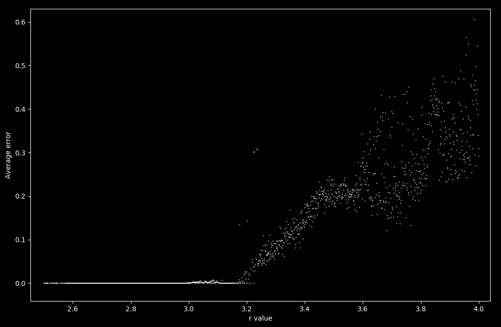
Do $r$ values yielding aperiodic iterations of \eqref{eq1} give worse estimates than $r$ values for periodic iterations of \eqref{eq1}? To get an idea of how this could be, let’s look at what happens to the average error as $r=2.5 \to r = 4$. The average error to any of the last four iterations may be found as follows:
Y = [] # list of average error per R value
R = [] # list of R values

for i in range(1500):
	r = 2.5 + i/1000
	starting_point = 0.5
	trajectory = [starting_point]
	for i in range(100):
		start = trajectory[-1]
		trajectory.append(r*start*(1-start))
	ls = [trajectory[-1]]
	s = set()
	steps = 100
	reverse_logistic_map(r, ls, steps, s)

	result_ls = [i for i in s]
	error_ls = []
	original_ls = []

	for i in range(len(result_ls)):
		error_ls.append(abs(logistic_map(r, result_ls[i], steps)-trajectory[-1]))
		original_ls.append(logistic_map(r, result_ls[i], steps))

	R.append(r)
	if len(error_ls) > 0:
		Y.append(sum([i for i in error_ls])/ len(error_ls))
	else:
		# if there are no previous values
		Y.append(-0.1) # some value that can be discarded

fig, ax = plt.subplots()
ax.plot(R, Y, '^', color='white', markersize=0.5)
ax.set(xlabel='r value', ylabel='Average error')
plt.show()
plt.close()
which results in the following plot.
If this is extended to the minimum error of any of the four last values of the trajectory from 0.5 in order to account for iteration error up to period 4, we instead have
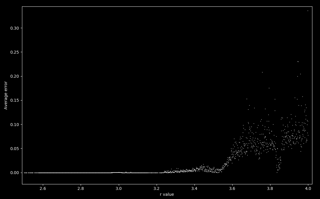
There is an increase in average error as the map becomes aperiodic, at around r = 3.58. This is to be expected for any value of r that yields a periodicity larger than 4, because iterations of either \eqref{eq1} or \eqref{eq2} are attracted to periodic orbits and the above program only takes into account accuracy up to four previous values (near four periodic values). As aperiodic trajectories have infinite period, the accuracy necessarily suffers.
To summarize, if the reverse logistic map is used to calculate values that result in accurate recapitulations of the intial value using the forward logistic map, error due to finding the right periodic trajectory but being on the ‘wrong’ iteration occurs because all periodic points are attractors. For r values giving an aperiodic trajectory of the forward logistic map, this error cannot be prevented because periodicity is infinite.
Some approximations of $x_{n-p}$ with \eqref{eq2} are necessarily better than others
The previous section saw some extimates of a previous value in the trajectory of the logistic map to yield more accurate vales of $x_n$ after p iterations of \eqref{eq1}. Is this necessarily the case, or in other words is there some way to compute the reverse logistic map such that all previous estimates are equivalently good?
Here is \eqref{eq2} restated for clarity:
\[x_{n+1} = \frac{r \pm \sqrt{r^2-4rx_n}}{2r}\]Now consider what many iterations of \eqref{eq2} entail, specifically that many square roots of $r^2-4rx_n$ are taken. For example,
\[x_{n+2} = \frac{r \pm \sqrt{r^2-4r(\frac{r \pm \sqrt{r^2-4rx_n}}{2r})}}{2r}\]Now some square roots are better approximated by rational numbers than others: most famously, the golden ratio $\phi = \frac{1 + \sqrt 5}{2}$ which is the positive root of $x^2-x-1$ is the irrational number that is ‘furthest’ from any rational in the sense that it is worst approximated by any rational. This can be shown with continued fractions:
\[\phi = 1 + \cfrac{1}{1+\cfrac{1}{1+\cfrac{1}{1+\cdots}}}\]Now consider what makes a poorly approximated number: if the denominator contains a large first integer before addition, then everything that follows is less important than if it were smaller. For example, see that $5 + \cfrac{1}{5 + \cfrac{1}{5}} \approx 5.19$ is better approximated by $5 + \cfrac{1}{5} = 5.2$ than $2 + \cfrac{1}{2 + \cfrac{1}{2}} = 2.4$ is by $2 + \cfrac{1}{2} = 2.5$ . With $1$ being the smallest non-zero natural number (and dividing by zero is unhelpful here) means that this number is most poorly approximated by ending this continued fraction at any finite stage. Approximation of the golden ratio is discussed in this excellent video from Numberphile.
Thus certain square root values are better approximated by rational numbers than others. Therefore, iterating \eqref{eq2} will yield numbers approximated better or worse depending on the value inside each radical, which in turn depends on whether addition or subtraction occurs at each iteration.
Now if the r value for \eqref{eq1} yields a periodic trajectory, \eqref{eq2} will be attracted to the same periodic trajectory and thus it does not matter whether addition or subtraction is chosen because either reaches the same value. But for aperiodic trajectories values never repeat, meaning that each choice for addition or subtraction in \eqref{eq2} yields unique values. Because different radicals are approximated by rational with differing success, and as computable procedures must use rational (finite) approximations, \eqref{eq2} must yield numbers that, when iterated with \eqref{eq1} to recover the original $x_0$, are of varying accuracy.
Aperiodic logistic maps are not practically reversible
The logistic map is not because it is 2-to-1 for many values of $x_n \in (0, 1)$: there is no way to know which of the two points $x_{n-1}, x_{n-1}’$ the trajectory actually visited. For values of r that yield an aperiodic logistic map trajectory, only one of the two $x_{n-1}, x_{n-1}’$ points may be visited because aperiodic trajectories never revisit previous points, and if either point was visited then $x_n$ is also visited. Therefore aperiodic logistic map trajectories follow only one of the many possible previous trajectories, and which one is impossible to determine.
But what about reversibility with respect to future values $(x_{n+1}, x_{n+2} …)$? In other words, given that $x_{n-1}, x_{n-1}’$ both map to the same trajectory $(x_{n+1}, x_{n+2} …)$, can we find any previous values of $x_n$ that yield the same fucutre trajectory? This criteria for reversibility is similar to the criteria for one-way functions, which stipulates that either $x_{n-1}, x_{n-1}’$ may be chosen as a suitable previous value and that there is no difference between the two with respect to where they end up. Is the logistic map reversible under this definition, or equivalently is the logistic map a one way function?
Symbolically, it is not: \eqref{eq2} may be applied any number of times to find the set of all possible values for any previous iteration. But if this is so, why was it so difficult to use this procedure to find accurate sets of previous values, as attempted in the last section?
Consider what happens when one attempts to compute successive iterations of \eqref{eq2}: first one square root is taken, then another and another etc. Now for nearly every initial value $x_n$, these square roots are not of perfect squares and therefore yield irrational numbers. Irrational numbers cannot be represented with complete accuracy in any computation procedure with finite memory, which certainly applies to any computation procedure known. The definition for ‘practical’ computation is precisely this: computations that can be accomplished with finite memory in a finite number of steps. The former stipulation is not found in the classic notion of a Turing machine, but is most accurate to what a non-analogue computer is capable of.
This would not matter much if approximations stayed accurate after many iterations of \eqref{eq2}, but one can show this to be untrue for values of r and $x_0$ such that \eqref{eq1} is aperiodic. First note that \eqref{eq2} forms a tree, with one $x_n$ leading to one or two $x_{n_1}$. If \eqref{eq1} is aperiodic for all starting $x_n$, then all paths through \eqref{eq2} are aperiodic because previous values are never revisited in the forward direction (with \eqref{eq1}), and therefore are never revisited in the reverse. Therefore all paths through \eqref{eq2} are sensitive to initial values (becase they are aperiodic) and it follows that any approximation of $x_n$ yields is arbitrarily inaccurate (within limites) for $x_{n+p}$ given a large enough $p$.
As iterations of \eqref{eq2} are (almost all) irrational, it follows that the reverse logistic map is impossible to compute practically (assuming aperiodicity) because finite representations of irrational numbers yield inaccurate estimates of future iterations.
The Henon map is invertible
The Henon map is a two dimensional discrete dynamical system defined as
\[x_{n+1} = 1 - ax_n^2 + y_n \\ y_{n+1} = bx_n \\ \tag{3} \label{eq3}\]Let’s try the same method used above to reverse $x_{n+1}$ of \eqref{eq2} with respect to time,
\[y_{n} = bx_{n+1} \\ x_{n+1} = \frac{y_n}{b}\]using this, we can invert $y_{n+1}$ as follows:
\[y_{n+1} = ax_{n+1}^2 + x_n - 1 \\ y_{n+1} = a \left(\frac{y_n}{b}\right)^2 + x_n - 1\]Therefore the inverse of the Henon map is:
\[x_{n+1} = \frac{y_n}{b} \\ y_{n+1} = a \left( \frac{y_n}{b} \right)^2 + x_n - 1 \tag{4} \label{eq4}\]This is a one-to-one map, meaning that \eqref{eq3} is invertible.
Does this mean that, given some point $(x, y)$ in the plane we can determine the path it took to get there? Let’s try this with the inverse function above for $a = 1.4, b=0.3$
#! python3
def reversed_henon_map(x, y, a, b):
	x_next = y / b
	y_next = a * (y / b)**2 + x - 1
	return x_next, y_next

array = [[0, 0]]
a, b = 1.4, 0.3
for i in range(4):
	array.append(reversed_henon_map(array[-1][0], array[-1][1], a, b))

print (array)
Starting at the origin, future iterations diverge extremely quickly:
[[0, 0], (0.0, -1.0), (-3.3333333333333335, 14.555555555555557), (48.518518518518526, 3291.331961591222), (10971.106538637407, 168511297.67350394)]
The reverse Henon map is unstable
We know that a starting value on the Henon attractor itself should stay bounded if \eqref{eq1} is iterated in reverse, at least for the number of iterations it has been located near the attractor. For example, the following yields a point that has existed near the attractor for 1000 iterations
def henon_map(x, y, a, b):
	x_next = 1 - a*x**2 + y
	y_next = b*x
	return x_next, y_next

x, y = 0, 0
a, b = 1.4, 0.3

for i in range(1000):
	x_next, y_next = henon_map(x, y, a, b)
	x, y = x_next, y_next

# x, y is the coordinate of a point existing near H for 1000 iterations
One might not expect this point to diverge until after the 1000 iterations have been reversed, but this is not the case: plugging x, y into the initial point for the reverse equation as follows
array = [[x, y]]
for i in range(30):
	array.append(reversed_henon_map(array[-1][0], array[-1][1], a, b))

print (array)
results in
[[0.5688254014690528, -0.08255572592986403], (-0.2751857530995468, -0.3251565203383966), (-1.0838550677946555, 0.36945277807827326), (1.231509260260911, 0.03940601355707107), (0.13135337852357026, 0.25566445433028995), (0.8522148477676332, 0.14813158398142479), (0.4937719466047493, 0.19354987712301397), (0.6451662570767133, 0.07650724558327537), (0.25502415194425126, -0.2637814976184484), (-0.8792716587281613, 0.3373902617238522), (1.1246342057461742, -0.10854872330010212), (-0.3618290776670071, 0.3079225997696742), (1.026408665898914, 0.11309157153833649), (0.37697190512778833, 0.225359610056858), (0.7511987001895267, 0.16699118716079653), (0.5566372905359884, 0.1849818026908716), (0.6166060089695721, 0.08892144895232601), (0.29640482984108674, -0.260395838616055), (-0.8679861287201833, 0.3511647173519976), (1.1705490578399922, 0.05027300681394742), (0.16757668937982473, 0.20986378339289535), (0.6995459446429846, -0.14731297048715142), (-0.4910432349571714, 0.03711878667906987), (0.12372928893023291, -1.469610723242318), (-4.898702410807727, 32.71992872244504), (109.06642907481681, 16647.781629174056), (55492.60543058019, 4311201068.530109), (14370670228.433699, 2.8912262794014697e+20), (9.637420931338232e+20, 1.3003183509091478e+42), (4.334394503030493e+42, 2.6301765991061335e+85), (8.767255330353778e+85, 1.0761067243866343e+172)]
which demonstrates divergence in around 22 iterations, far fewer than the 1000 iterations that were performed by the Henon map in the forward direction to reach the initial point.
Could this be due to propegation of error? Supposing a sufficiently small error $\varepsilon$ were added to both $y_n, x_n$, after one iteration of the reverse Henon map we have:
\[x_{(n+1)'} = (y_n + \varepsilon)/b \\ y_{(n+1)'} = \frac{a}{b^2}(y_n^2 + 2y_n\varepsilon + \varepsilon^2) + x_n + \varepsilon - 1 \\\]Now for the attractor that forms given $a = 1.4, b = 0.3$, we know that $\lvert y_n \rvert < 1/2$. Using this information, the distance between $x_{n+1}, y_{n+1}$ and $x_{(n+1)’}, y_{(n+1)’}$ can be calculated to see how much larger the error gets after each iteration of the inverse Henon map. We will use Manhattan distance (which is $\lvert x_1 - x_2 \rvert + \lvert y_1 - y_2 \rvert$) as our metric for simplicity.
This distance can be calculated, assuming $\varepsilon < 1$ such that $\varepsilon^2 < \varepsilon$, as follows:
\[\lvert x_{n+1} - x_{(n+1)'} \rvert + \lvert y_{n+1} - y_{(n+1)'} \rvert \\ = \frac{\varepsilon}{b} + \frac{a}{b^2}(2y_n\varepsilon + \varepsilon^2) + \varepsilon \\ < \frac{10}{3}\varepsilon + \frac{2\varepsilon}{10} + \varepsilon \\ < 10\varepsilon\]Therefore the Manhattan distance between the next point with compared to the point without error is less than 10-fold the initial error size for each iteration. Therefore a 100-fold increase in error requires more than 2 iterations. Now comparing back to our points with ~16 decimal places, we can say that the error will remain relatively small as long as the iteration number is under 16, but after this iteration the initial error introduced by rounding starts to become large relative to the point’s values.
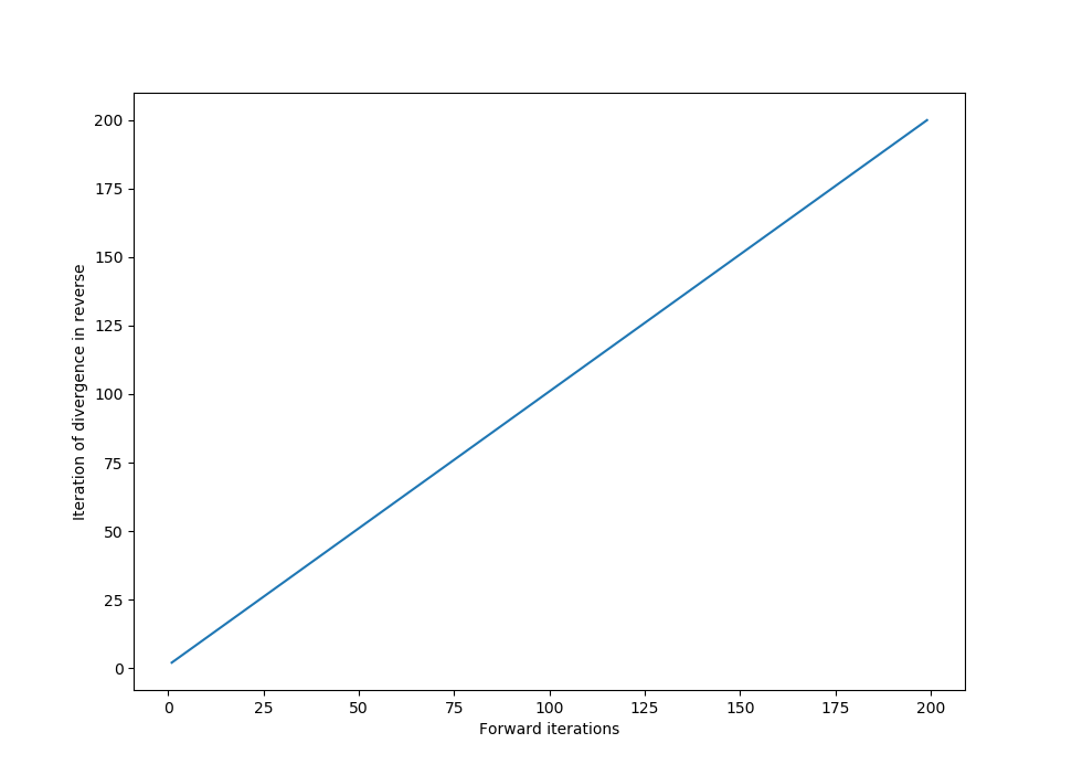
All this is to say that the divergence above occurred after 22 iterations because there were only ~16 decimal points of accuracy. What happens when this accuracy is increased? Arbitrary precision (within memory and time limits, that is) math can be performed using the decimal library. To find the number of iterations (in the inverse Henon map) until divergence (given 2000 forward iterations) at various decimal accuracies,
import numpy as np
from matplotlib import pyplot as plt
import copy
from decimal import *

# applies to an external x, y value or array
def reversed_henon_map(x, y, a, b):
	x_next = y / b
	y_next = a * (y / b)**Decimal(2) + x - Decimal(1)
	return x_next, y_next

# the forward Henon map for accuracy checking
def henon_map(x, y, a, b):
	x_next = Decimal(1) - a*x**Decimal(2)+ y
	y_next = b*x
	return x_next, y_next

x_array, y_array = [], []

for i in range(2, 1000):
	getcontext().prec = i
	x, y = Decimal(1), Decimal(1)
	a, b = Decimal(14)/Decimal(10), Decimal(3)/Decimal(10)

	for j in range(2000):
		x_next, y_next = henon_map(x, y, a, b)
		x, y = x_next, y_next
	x_array.append(i)

	count = 0
	while True:
		x, y = reversed_henon_map(x, y, a, b)
		if x > 100 or y > 100:
			break
		count += 1
	y_array.append(count)
yields
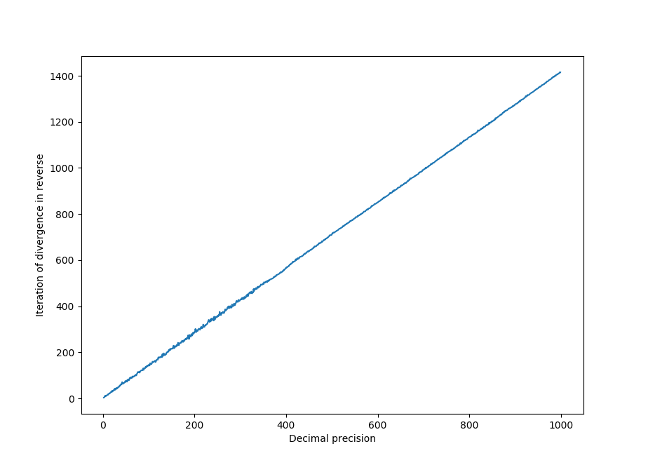
From this we can see that there is a linear relation between how many iterations it takes to diverge in the reverse direction and the precision used. This is because with more precision, we can better approximate values of points on the true Henon map (which are irrational for $a, b$ values that yield an aperiodic attractor, see below for more).
What happens to the number of reverse iterations until divergence if the precision is held constant (at 1000 decimal points) but the number of forward iterations changes?
Which is what we would expect, as each forward iteration (within the limits prescribed by the accuracy of calculation) brings the point closer to $\mathscr H$ at the same rate as a reverse iteration moves the point away from $\mathscr H$.
Stable and unstable points of the inverted Henon map
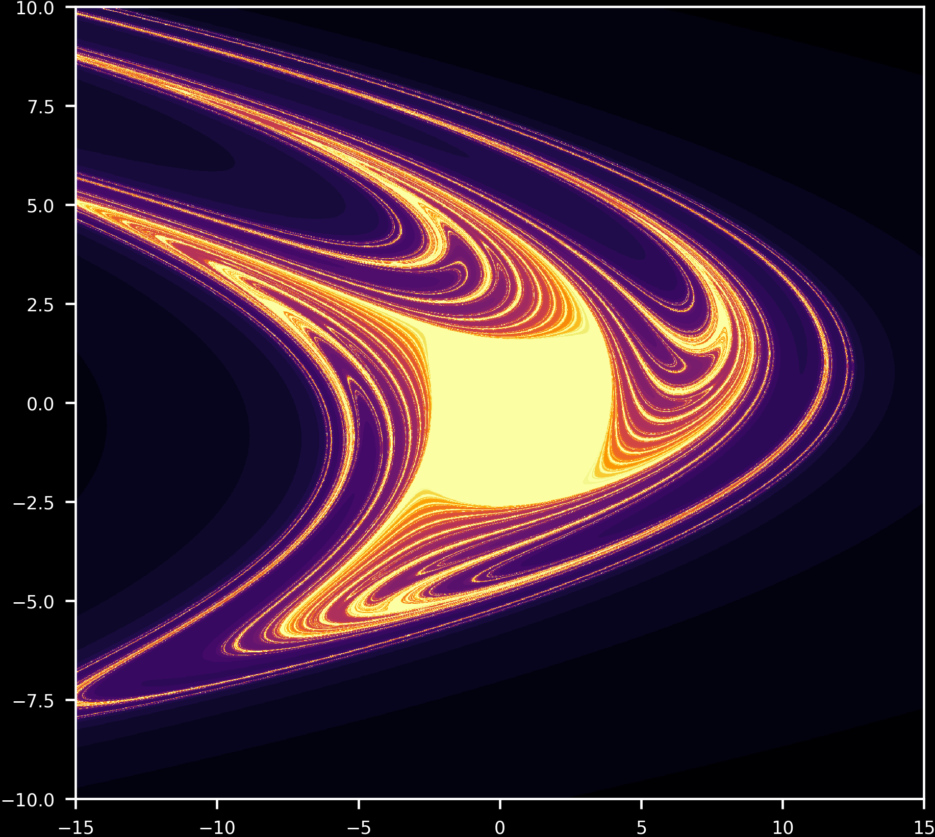
Is the divergence specific to the point we chose above, or do all points near the Henon attractor eventually diverge in a similar manner? This can be investigated as follows:
def reverse_henon_stability(max_iterations, a, b, x_range, y_range):
	xl, xr = -2.8, 2.8
	yl, yr = 0.8, -0.8

	x_list = np.arange(xl, xr, (xr - xl)/x_range)
	y_list = np.arange(yl, yr, -(yl - yr)/y_range)
	array = np.meshgrid(x_list[:x_range], y_list[:y_range])

	x2 = np.zeros(x_range)
	y2 = np.zeros(y_range)
	iterations_until_divergence = np.meshgrid(x2, y2)

	for i in iterations_until_divergence:
		for j in i:
			j += max_iterations

	not_already_diverged = np.ones(np.shape(iterations_until_divergence))
	not_already_diverged = not_already_diverged[0] < 1000

	for k in range(max_iterations):
		x_array_copied = copy.deepcopy(array[0]) # copy array to prevent premature modification of x array

		# henon map applied to array
		array[0] = array[1] / b
		array[1] = a * (array[1] / b)**2 + x_array_copied - 1

		r = (array[0]**2 + array[1]**2)**0.5
		diverging = (r > 10000) & not_already_diverged # arbitrarily large number here
		not_already_diverged = np.invert(diverging) & not_already_diverged
		iterations_until_divergence[0][diverging] = k

	return iterations_until_divergence[0]
which results (lighter color indicates more iterations occur before divergence)
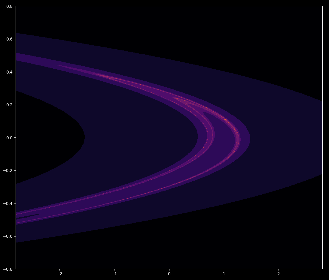
The baker’s dough topology found by Smale is evident in this image, meaning that each iteration of the forward Henon map can be decomposed into a series of three stretching or folding events as shown here. This topology is common for attractors that map a 2D surface to an attractor of 1 < D < 2: the Henon map for a=1.4, b=0.3 is around 1.25 dimensional.
The attractor for \eqref{eq3} can be mapped on top of the divergence map for \eqref{eq4} as follows:
steps = 100000
X = [0 for i in range(steps)]
Y = [0 for i in range(steps)]

X[0], Y[0] = 0, 0 # initial point

for i in range(steps-1):
	if abs(X[i] + Y[i])**2 < 1000:
		X[i+1] = henon_map(X[i], Y[i], a, b)[0]
		Y[i+1] = henon_map(X[i], Y[i], a, b)[1]

plt.plot(X, Y, ',', color='white', alpha = 0.5, markersize = 0.1)
plt.imshow(reverse_henon_stability(40, a, b, x_range=2000, y_range=1558), extent=[-2.8, 2.8, -0.8, 0.8], aspect= 2.2, cmap='inferno', alpha=1)
plt.axis('off')
plt.savefig('henon_reversed{0:03d}.png'.format(t), dpi=420, bbox_inches='tight', pad_inches=0)
plt.close()
which gives

where, as expected, the areas of slower divergence align with the attractor (in white).
From a = 1 to a = 1.5, holding b=0.3 constant,
It is interesting to note that the divergence map for the forward Henon map \eqref{eq3} is not simply the inverse of the divergence map for the reverse Henon map \eqref{eq4}, which is presented here, given that they are inverse functions of each other. In particular, regions outside the attractor basin for \eqref{eq3} diverge, meaning that a trajectory starting at say (10, 10) heads to infinity. But this region also diverges for \eqref{eq4}, which is somewhat counter-intuitive given that \eqref{eq4} yields the iterations of \eqref{eq3} in reverse.
For a=0.2, -1 < b < 0, \eqref{eq3} experiences a point attractor for initial values in the attractor basin: successive iterations spiral in towards the point
\[x_n = \frac{(b-1) + \sqrt{(b-1)^2 + 4a}}{2a} \\ y_n = bx_n\]outside of which values diverge. For b <= -1, the attractor basin collapses, and nearly all starting points lead to trajectories that spiral out to infinity. Now looking at stable versus unstable values for \eqref{eq4} with b = -0.99,
The area in the center does not diverge after 40 iterations. Do initial points in this area ever diverge? This question can be addressed by increasing the maximum iterations number. Doing so from 2 maximum iterations to 1010, iterating \eqref{eq4} for a=0.2, b=-0.99 we have
As is the case for a=1.4, b=0.3 so also for \eqref{eq3} with a=0.2, b=-0.99, there are unstable points and regions elsewhere diverge.
The transition from point attractors to divergence everywere except a point (or two) for the reverse Henon map occurs in reverse to that observed for the forward Henon. For example, a=0.2 and b=0.95 exhibits two point attractors for \eqref{eq3} but diverges everywhere except unstable points for \eqref{eq4}, whereas a=0.2, b=1.05 diverges everywhere except unstable points for \eqref{eq3} but converges on points for \eqref{eq4}. In the video below, $a$ is held constant while $b$ changes as follows:
\[a = 0.2 \\ b = 0.95 \to b = 1.01\]Iterating \eqref{eq4}, note how the change in basin behavior is the opposite to that found for the same transition with \eqref{eq3}.
Aperiodic Henon maps are reversible from some starting points
Is the Henon map reversible? In the sense that we can define a composition of functions to determine where a previous point in a trajectory was located, the Henon map is reversible as it is 1-to-1 and an inverse function exists. Reversing the Henon map entails computing \eqref{eq3} for however many reverse iterations are required.
But earlier our attempts to reverse the Henon map were met with very limited success: values eventually diverged to infinity even if they were located very near the attractor for \eqref{eq3}. Moreover, divergence occurred in fewer iterations that were taken in the original forward trajectory. This begs the question: is the Henon map, like the logistic map, practically irreversible?
If it is aperiodic (as is the case for a=1.4, b=0.3) then yes, for the special case where the point of interest is an element of the set of points in the Henon attractor $\mathscr H$, in symbols $x_n \in \mathscr H$, or more generally where $x_n \not \in \Bbb Q$. The Henon map, iterated discontinuously, cannot be defined on the rationals (for more information, see here). As real numbers are uncountably infinite but rationals are countable, all but a negligable portion of values of the Henon attractor $\mathscr H$ are irrational.
Now irrational numbers are of infinite length, and cannot be stored to perfect accuracy in finite memory. How do we know that rational approximations of irrational numbers eventually diverge after many iterations of \eqref{eq4}? This is because of sensitivity to initial conditions, which implies and is implied by aperiodicity (see here). The proof that \eqref{eq4} is sensitive to initial conditions is as follows: \eqref{eq4} is the one-to-one inverse of \eqref{eq3}. Being aperiodic, the trajectory of \eqref{eq3} never revisits a previous point. Therefore we know that \eqref{eq4} is aperiodic as well, as it never revisits a previous point being that it defines the same trajectory as \eqref{eq3}. As aperiodicity implies arbitrary sensitivity to initial values, \eqref{eq4} is arbitrarily sensitive to initial values.
Any two starting points $p_1$ and $p_2$, arbitrarily close together but not exactly in the same place, can be considered approximations of each other. If they are close enough then they are accurate approximations. Sensitivity to initial conditions stipulates that, given enough iterations of the inverse Henon map \eqref{eq4}, $p_1$ and $p_2$ will separate. If we take $p_1$ to be an irrational number and $p_2$ to be its rational approximation (or vice versa), an arbitrarily accurate rational approximation will, given enough iterations of \eqref{eq4}, become inaccurate. Therefore all but a negligable portion of values on an aperiodic Henon map itself are practically non-invertible.
One might expect for the errors introduced in approximating irrationals in one direction with respect to time to cancel out if the reverse function is used to back-compute in the other direction. If this were true, then even though iterations of \eqref{eq4} do not give accurate previous values beyond a certain number of iterations, the function would still be reversible in the sense of a one-way function definition (see the discussion for the logistic map for more on this topic) because either the true value or its inaccurate approximation (which is computed) would yield the same point. But even though tempting, the idea that perhaps errors should cancel each other out can easily be disproven for aperiodic 1-to-1 dynamical systems as follows: if a true value and an inaccurate approximation cannot both yield the same point in reverse because otherwise the system would be 2-to-1, a contradiction.
The last statement does not necessarily mean that \eqref{eq3} is not practically invertible for periodic trajectories, because any finite number of iterations of \eqref{eq3} could still be reversed with the same number of iterations of \eqref{eq4}.
What about if we start with a rational number not on the Henon attractor itself, given such an $x_n$ can we find $x_{n-p}$? Given sufficient memory the Henon map is reversible for such points, as \eqref{eq4} is closed for rationals. This means that in contrast to what we saw for the logistic map, the Henon map starting on a rational $x_n$ is reversible. But memory demands are exponential as iterations increase.
Aperiodicity and reversibility
In conclusion, aperiodic Henon but not logistic maps are practically reversible for some starting value, meaning that one cannot compute arbitrary previous values accurately using finite memory.
If future values for the logistic map are difficult to predict, as is the case for aperiodic systems in general, does it come as any surprise that past values are hard to determine as well? It is indeed surprising, but why this is requires explanation.
First consider what it means for an aperiodic dynamical system to be hard to predict. More precisely, it is often stated that the approximate present does not determine the approximate future, which is a consequence of sensitivity to initial values. But it should be understood that the exact present does indeed determine the exact future: every time \eqref{eq1} is iterated 30 times with idential (rational) starting values for a fixed r, the result is the same (assuming identical floating point arithmetic). Real observations are necessarily imperfect, but if a rational value is used as a starting point to iterate the logistic equation then all future iterations are computable, given enough memory.
On the other hand, this page demonstrates a separate difficulty in attempting to calculate previous values from the logistic map. Choosing a rational value of $x_n$ is no guarantee that any previous value will be rational, and sensitivity to initial values necessitates that small approximation errors become large over time. This means that no computation procedure with finite memory will be able to accurately determine past values for an arbitrary number of iterations, regardless of starting value. The logistic map, therefore, is deterministic and computable in the forward time direction (given the right starting values and enough memory) but not in the reverse time direction.