The boundary of the logistic map

The logistic map is a conjugate of a Julia set

The logistic equation

\[x_{n+1} = rx_n (1 - x_n) \\ \tag{1} \label{eq1}\]

is a model for growth rate that displays many features of nonlinear dynamics in a nice one-dimensional form. For a summary on some of these interesting properties, see here.

Why aren’t values for r>4 shown in any of the graphs for the logistic equation? This is because these values head towards infinity: they are unbounded. Which values are bounded? This question is not too difficult to answer: for r values of 0 to 4, initial populations anywhere in the range $[0, 1]$ stay in this range.

What if we iterate \eqref{eq1} but instead of $x$ existing on the real line, we allow it to traverse the complex plane? Then we have

\[z_{n+1} = rz_n (1 - z_n) \\ \tag{2} \label{eq2}\]

Where $z_n$ (and thus $z_{n+a}$ for any $a$) and $r$ are points in the complex plane using the Gaussian plane:

\[z_n = x + yi \\ r = x + yi\]

Now which points remain bounded and which head towards infinity? Let’s try fixing $r$ in place, say at $3$ and seeing what happens to different starting points in the complex plane after iterations of \eqref{eq3}.

The result looks very similar to a Julia set, is defined as the set of points bordering initial points whose subsequent iterations of

\[z_{n+1} = z_n^2 + c \tag{3} \label{eq3}\]

that diverge (head to infinity) and points whose subsequent interations do not diverge.

For $c = -0.75 + 0i$, this set is shown below (with an inverted color scheme to that used for the logistic map for clarity)

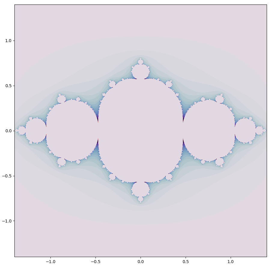
These maps look extremely similar, so could they actually be the same? They are indeed! The logistic map \eqref{eq1} and the quadratic map \eqref{eq3} which forms the basis of the Julia sets are conjugates of one another: they contain identical topological properties for a certain $a$ value, or in other words transforming from one map to another is a homeomorphism.

This can be shown as follows: a linear transformation on any variable is the same as a (combination of) stretching, rotation, translation, or dilation. Each of these possibilities does not affect the underlying topology of the transformed space, which one can think of as being true because the space is not broken apart in any way.

This being the case, if it is possible to transform the logistic map \eqref{eq1} into the quadratic map \eqref{eq3} with the linear transformation $h(x) = ax+b$, then these maps are topologically equivalent. To test this, with the following definitions for the logistic and quadratic equations,

\[f(x) = rx(1-x) \\ g(x) = x^2 + c \\\]

is there some linear transformation

\[h(x) = ax+b\]

that makes

\[h(f(x)) = g(h(x))\]

true?

This can be expanded for clarity:

\[a(rx_n(1-x_n)) + b = (ax_n + b)^2 + c \\ arx_n - arx_n^2 + b = a^2x_n^2 + 2abx_n + b^2 + c \\\]

and now substituting useful values for $a$ and $b$ to remove terms,

\[b = r/2 \implies -arx_n^2 + b = a^2x_n^2 + b^2 + c \\ a = -r \implies b = b^2 + c \\ c = b - b^2\]

putting these expressions together, the conjugacy is valid whenever

\[c = \frac{r}{2} \left( 1-\frac{r}{2} \right)\]

Therefore the quadratic map is by a homeomorphism (in particular, a linear transformation) equivalent to the logistic map, and thus the two are topologically equivalent. Now the necessity of the seemingly arbitrary value of $a=-0.75$ for the Julia set above is clear: $r=3$ was specified for the logistic map, and by our homeomorphism then $c= \frac{3}{2}(1-\frac{3}{2}) = -3/4$.

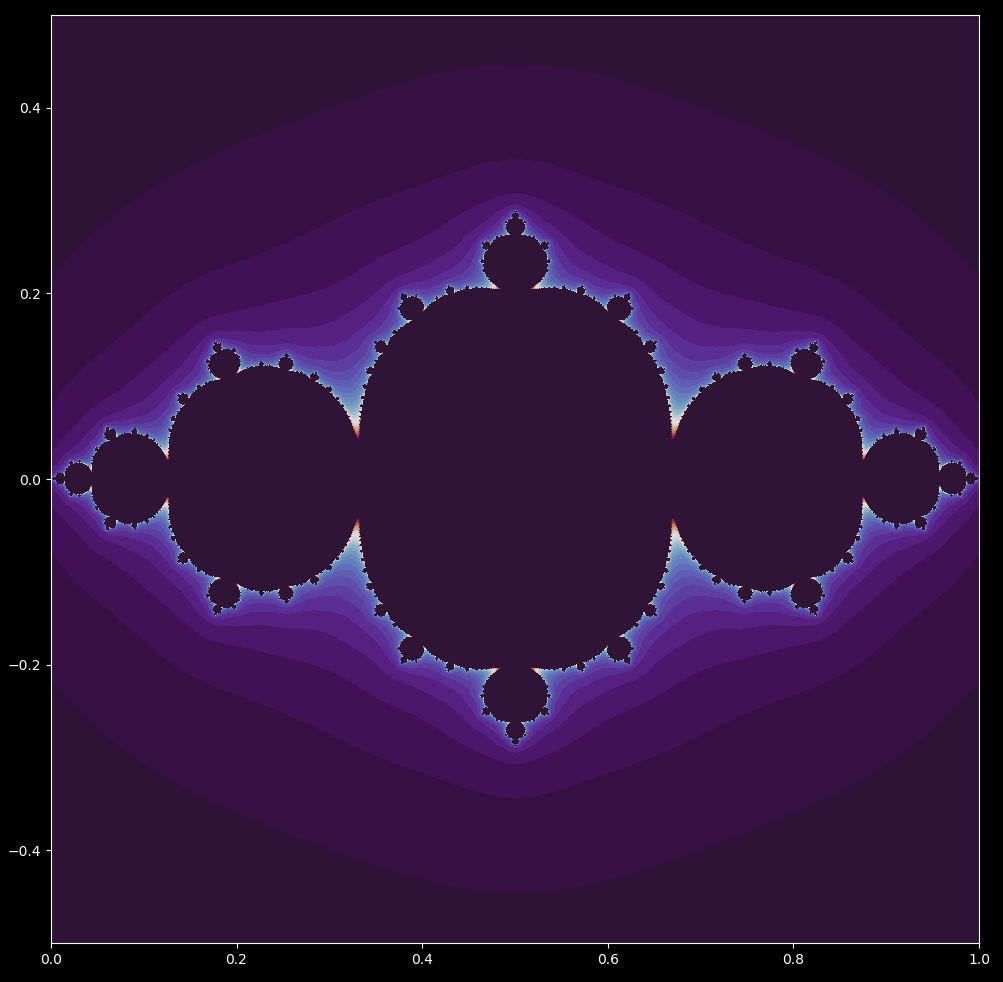
All this is to say that for any $r$ value, the logistic map is equivalent to a Julia set where $c=\frac{r}{2}(1-\frac{r}{2})$. Just for fun, let’s zoom in on the logistic boundary map above, focusing on the origin.

An aside: for most decreases in scale, more iterations are required in order to determine if close-together coordinates will diverge towards infinity or else remain bounded. But this is not the case for a zoom towards the origin: no more iterations are required for constant resolution even when the scale has increased by a factor of $2^{20}$.

The logistic map and the Mandelbrot set

Julia sets may be connected or disconnected. As the logistic map \eqref{eq1} is a homeomorphism of the quadratic map Julia set \eqref{eq3}, identical set topologies should be observed for the logistic map. Observing which values $z_0$ border bounded and unbounded iterations of the logistic map in the complex plane

\[z_{n+1} = rz_n(1-z_n) \tag{2}\]

from $r=2 \to r=4$ (both on the real line) for the logistic map, we have

This is analagous to observing Julia sets where $c=0 \to c=-2$.

What happens if we instead fix the starting point and instead plot the points $r = x + yi$ for which the logistic map \eqref{eq2} diverges versus points that do not diverge? For the starting point $z_0 = 1/2 + 0i$, we get

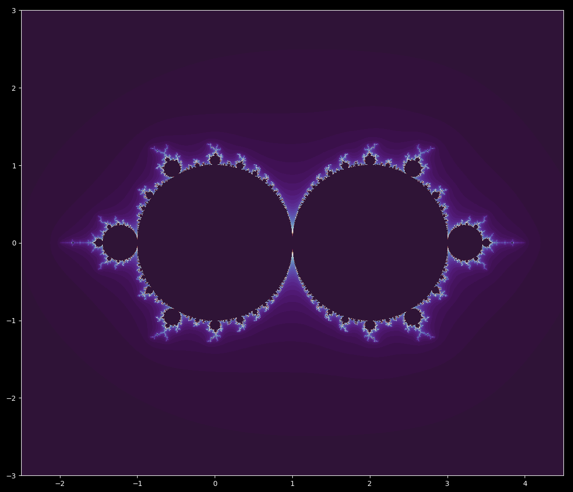
This figure resembles a double-sided Mandelbrot set. When we zoom in, we can find many little mandelbrot sets (in reversed x-orientation). The Mandelbrot set is the map where the initial value $z_0$ is fixed at the origin and the points for which $c$ diverge or not are potted. This is analagous to fixing the starting point for the logistic equation and then looking at which $r$ values cause future iterations to diverge using the $c=r/2(1-r/2)$ found above:

\[z_{next} = z_n^2 + \frac{r}{2} \left( 1-\frac{r}{2} \right) \tag{4}\]

For $z_0 = 0+0i$, this is identical to the logistic map above (which stipulates the starting point $z_0 = 1/2 + 0i$ is not at the origin).

Why are the starting points different for these maps, even though the output is the same? If one iterates the logistic map from point $x_0 = 0+0i$, no value of $r$ will cause the trajectory to diverge (as it stays at the origin). Observing the Julia set and logistic set above, it is clear that the map has been translated by $1/2 + 0i$ units and has also been compressed. This is true for any Julia set with an equivalent logistic set, which is why we have to start at $1/2 + 0i$ for the latter to make an identical Mandelbrot set to the former.

To make identical maps for any one starting point $z_0 = x + yi$, we may use the homeomorphic functions (see above) before the change of variables which are

\[a(rx_n(1-x_n))+b \\ (ax_n+b)^2 + c \\ a=r/2, \; b=-r,\; c=\frac{r}{2} \left( 1-\frac{r}{2} \right)\]

Iterating either equation gives the same map of converging versus diverging iterations for various $r$ values in the complex plane for any starting value $z_0$. For example, $z_0 = 1/4$ gives

Zoom and extended logistic set

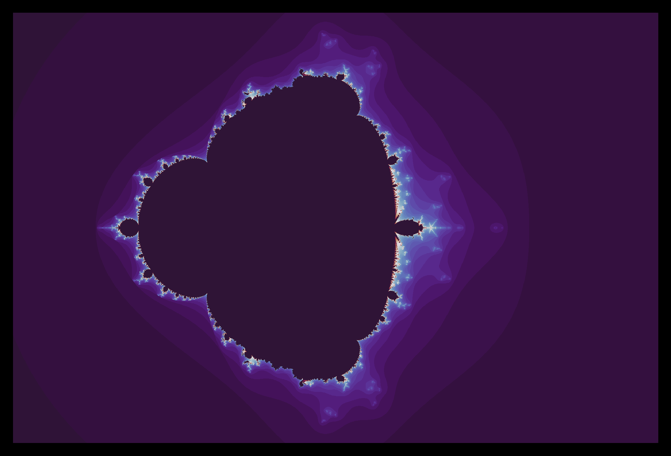
The Mandelbrot set is well known for its fractal structure that yields interesting patterns at arbitrary scale. The logistic map boundary is the same in this respect: for example, increasing scale at the point

\[(3.58355 + 0i)\]

yields

Note the identical objects found in a Mandelbrot set zoom on the point

\[(-1.633 + 0i)\]

A programmatic aside: the previous and following zooms were made using a different method than elaborate on previously. Rather than modifying the ogrid directly, a_array and z_array are instead positioned (using addition and subtraction of real and imaginary amounts) and then scaled over time as follows:

def mandelbrot_set(h_range, w_range, max_iterations, t):
	y, x = np.ogrid[1.4: -1.4: h_range*1j, -1.8: 1:w_range*1j] # note that the ogrid does not scale

	a_array = x/(2**(t/15)) - 1.633 + y*1j / (2**(t/15)) # the array scales instead
	z_array = np.zeros(a_array.shape)
	iterations_till_divergence = max_iterations + np.zeros(a_array.shape)
  
  ...

This method requires far fewer iterations at a given scale for an arbitrary resolution relative to the method of scaling the ogrid directly, although more iterations are required for constant resolution as the scale decreases. The fewer iteration number necessary is presumably due to decreased round-off error: centering the array and zooming in on the origin leads to approximately constant round-off error, whereas zooming in on a point far from the origin leads to significant error that requires more iterations to resolve. I am not completely certain why a constant number of iterations are not sufficient for constant resolution using this method, however.

Also as for the Mandelbrot set, we can change the map by changing the starting point of the logistic map \eqref{eq2}. For example, moving the starting point from $x_0 = 0 \to x_0 = 2$ yields