Pendulum map

Imagine a pendulum swinging back and forth. We can plot the position of its tip on the x-axis and the velocity of the tip on the y-axis. This xy plane is now called a phase space, and although it does not correspond to physical space it does tell us interesting information about the system it represents. An excellent summary of modeling differential equations by 3B1B may be found here.

By setting up a pendulum to obey Newton’s laws, we can model how the pendulum will swing using Euler’s formula to model the trajectory through phase space of the differential equations governing pendulum motion as it is slowed by friction:

\[\cfrac{dx}{dt} = y \\ \cfrac{dy}{dt} = -ay - b \cdot \sin(x) \tag{1}\]

Where the constant $a$ denotes friction and the constant $b$ represents the constant of gravity divided by the length of the pendulum. This system of equations is nonlinear (due to the sine term) and dissipative (from the friction, $-ay$) which means that it takes a 2D volume of starting points down to a 0 area.

It is helpful to view the vector plot for this differential system to get an idea of where a point moves at any given (x,y) coordinate:

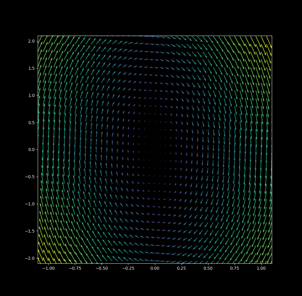
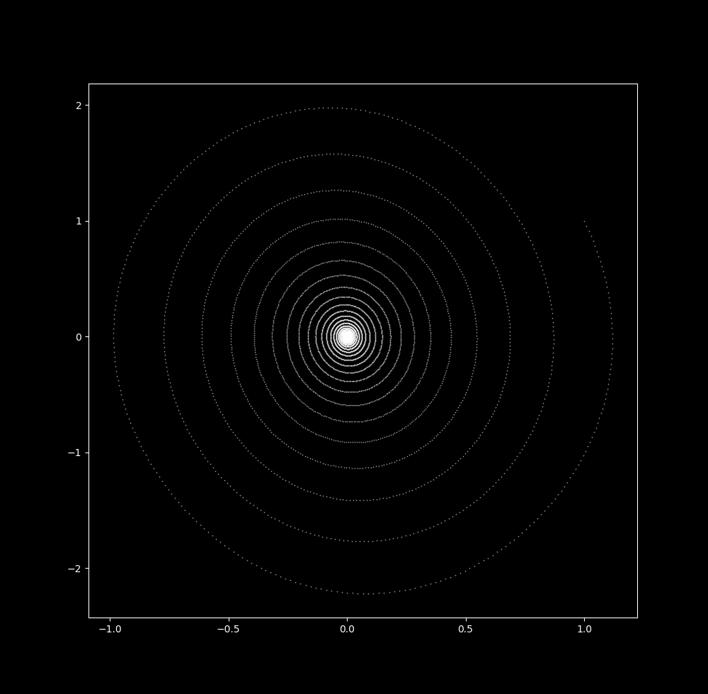
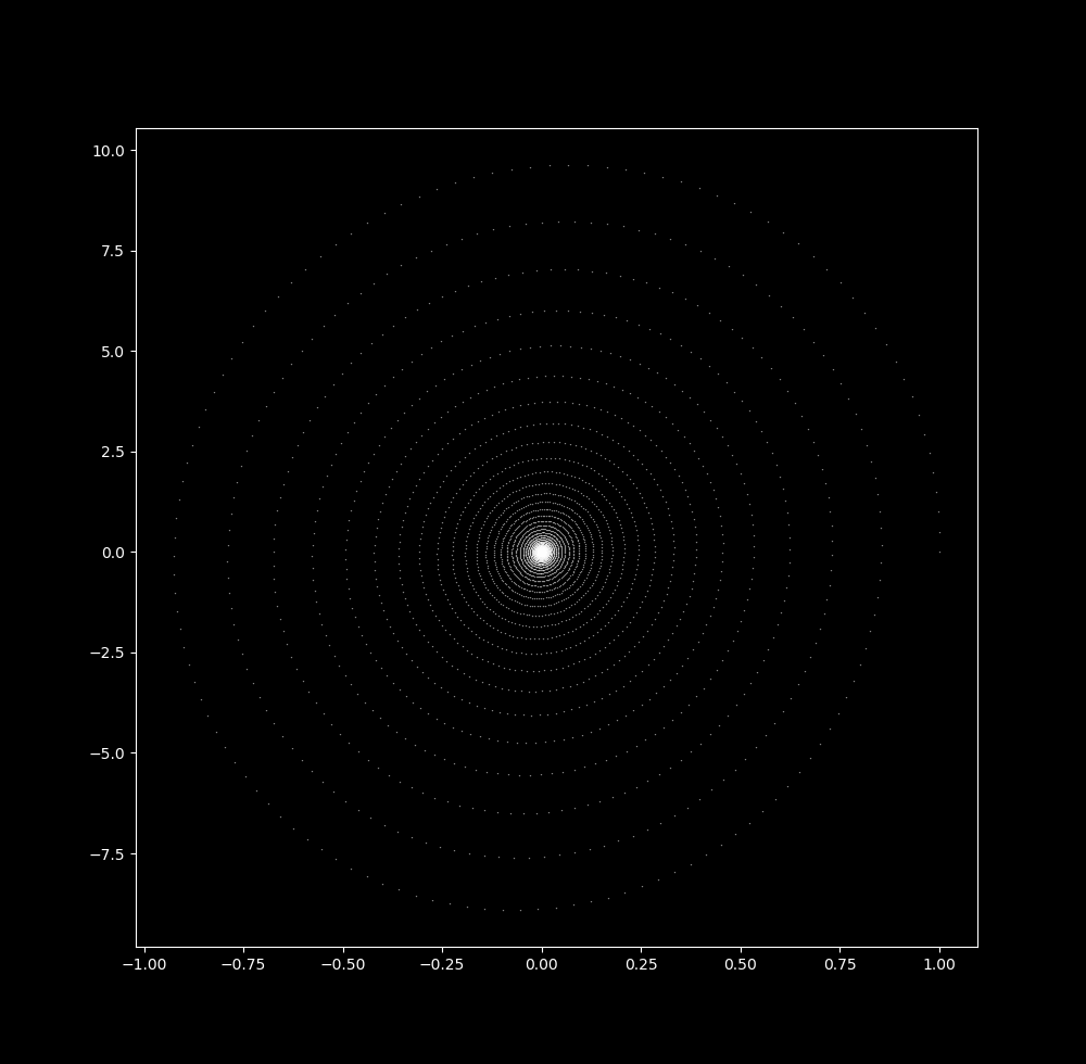
Imagine a ball rolling around on a plane that is directed by the vectors above. We can calculate this rolling using Euler’s formula (see here) the change in time step $\Delta t$ is small (0.01 in this case), the following map is produced:

Now note that we can achieve a similar map with a linear dissipative differential system

\[\cfrac{dx}{dt} = -ay \\ \cfrac{dy}{dt} = -by + x \tag{2}\]

which at $\Delta t = 0.1 $ yields

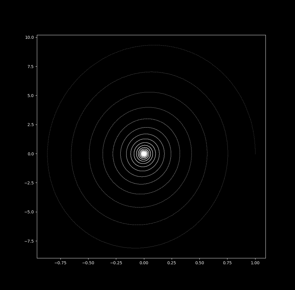
In either case, the trajectory heads asymptotically towards the origin. This is also true for any initial point in the vicinity of the origin, making the point (0,0) an attractor of the system. As the attractor is a point, it is a 0-dimensional attractor or point attractor.

Increasing timestep size leads to an increase in attractor dimension

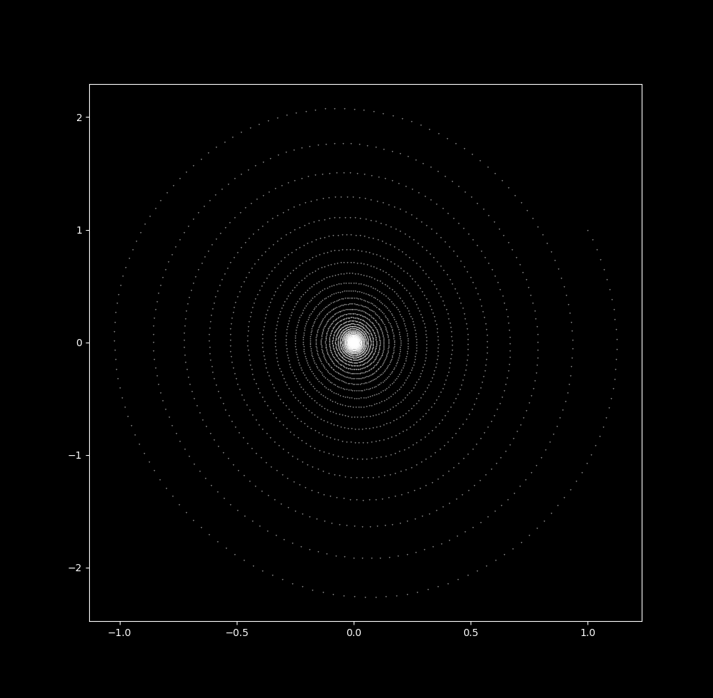
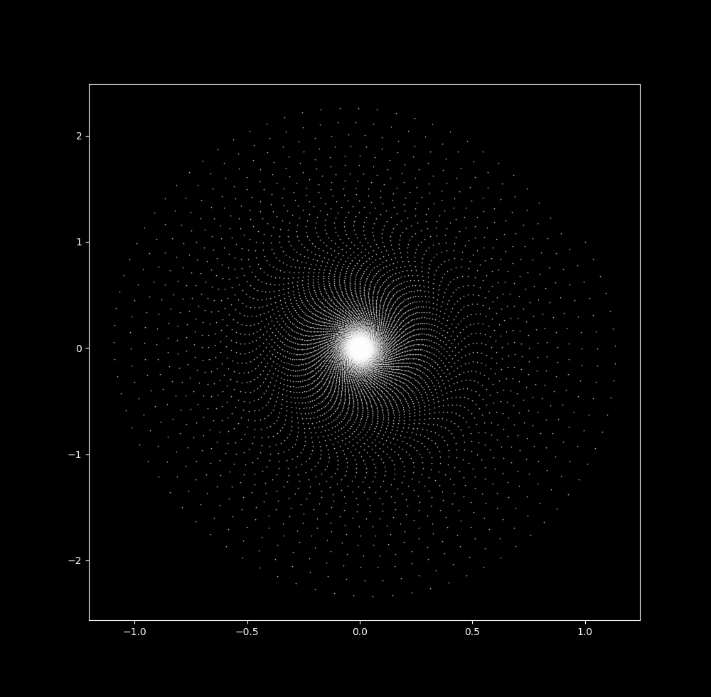
Now let’s increase $\Delta t$ little by little. At $\Delta t = 0.02$ the map looks similar to the one above just with more space betwen each point on the spiral. This makes sense, as an increase in timestep size would lead to more motion between iterations provided a particle is in motion.

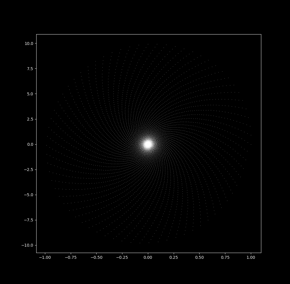
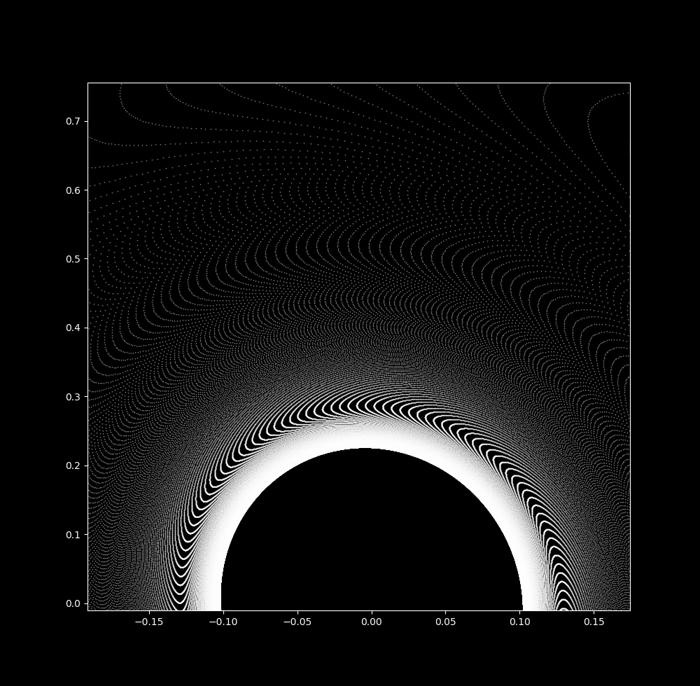
Increasing $\Delta t$ to 0.037 leads to the appearance of ripples in the trajectory path, where the ratio between the distance between consecutive iteration (x, y) coordinates compared to the (x, y) coordinates of the next nearest neighbor changes depending on where in the trajectory the particle is. For lack of a better word, let’s call these waves. Another way to think about the waves is to see that they are locations of apparent changes in spiral direction.

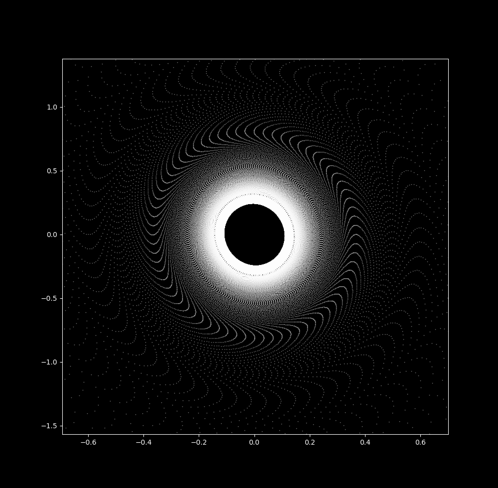
With a slightly larger $\Delta t$ (0.04088), the waves have become more pronounced and an empty space appears around the origin (picture is zoomed slightly).

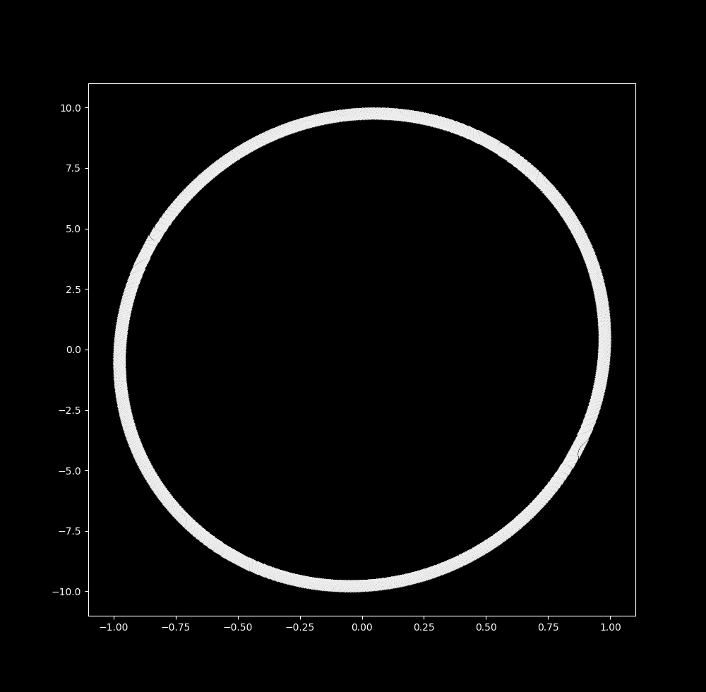
And by $\Delta t = 0.045$, the attractor is now a ring

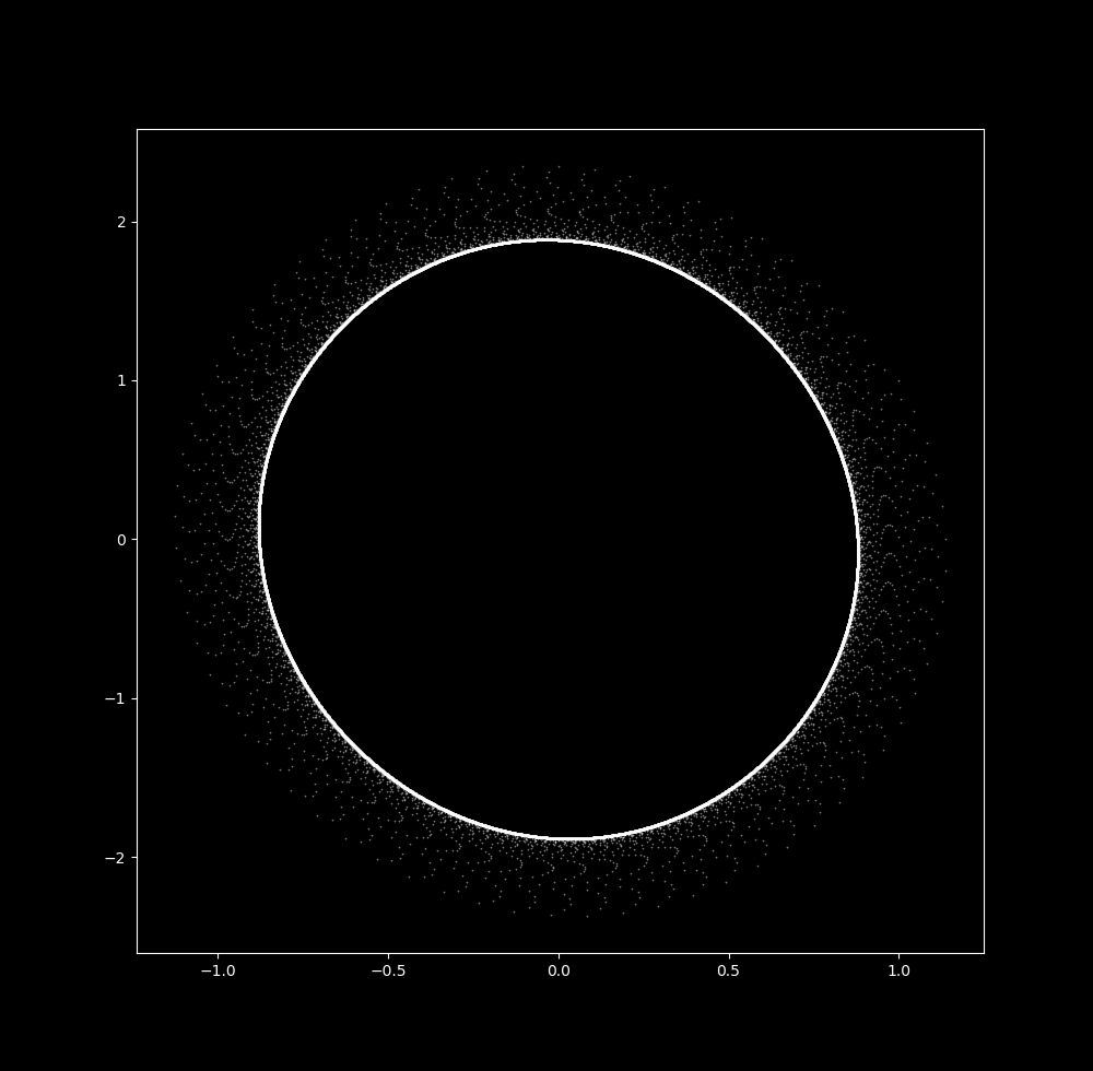
Thus an increase in $\Delta t$ leads to the transformation of the pendulum map from a 0-dimensional attractor to a 1-dimensional one. Further increases in $\Delta t$ leads to explosion towards infinity.

Here is a video of the transition from $\Delta t = 0.03 \to \Delta t = 0.045$:

What happens to the linear system (2) when $\Delta t$ increases? At $\Delta t = 0.5$, the points along the spiral are slightly more spaced out

When $\Delta t = 0.9$, there is less space between (x, y) coordinates of different rotations than of consecutive iterations:

And when $\Delta t = 0.9999$, this effect is so pronounced that there appears to be a ring attractor,

But this is not so! Closer inspection of this ring reveals that there is no change in point density between the starting and ending ring: instead, meaning that the points are still moving towards the origin at a constant rate.

Only at $\Delta t = 1$ is there a 1-dimensional attractor, but this is unstable: at small values less than or greater than 1, iterations head towards the origin or else towards infinity. The linear system yields a 1-dimensional ring map only when the starting coordinate is already on the ring, and thus it is incapable of forming a 1-dimensional attractor (ie a stable set) as was the case for the nonlinear system.

From $\Delta t = 0.9 \to \Delta t = 0.999$,

Eventually periodic pendulum map

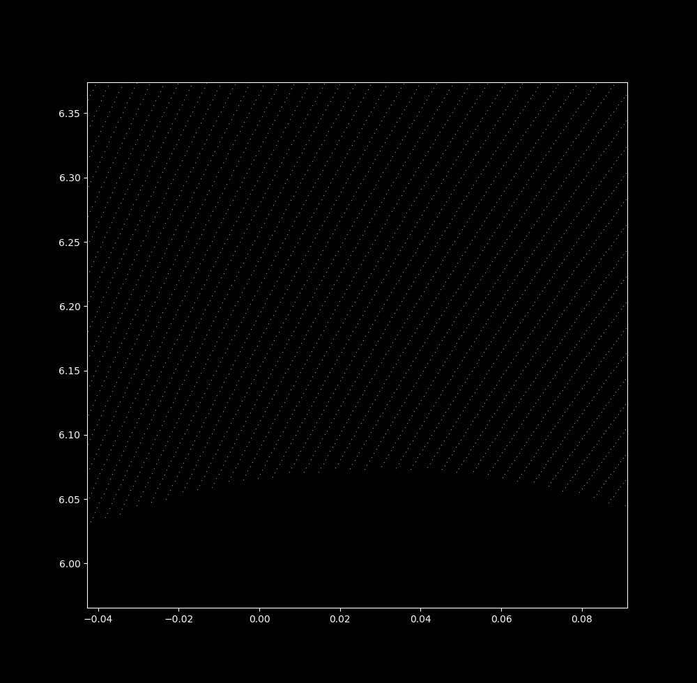
Take $\Delta t$ to be 0.04087. Now let’s zoom in on the upper part of the map:

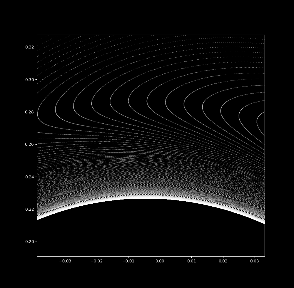
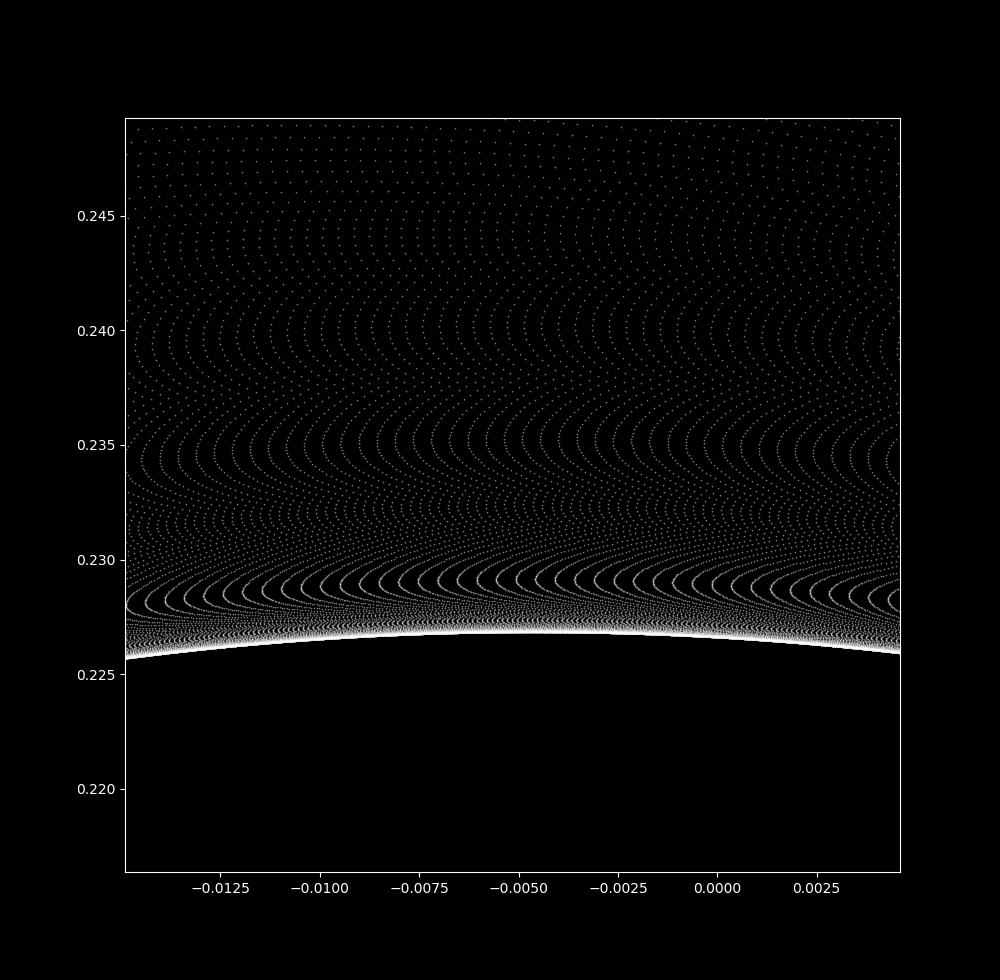
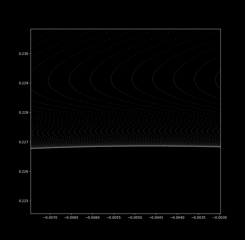
Notice that more and more waves are visible as the scale decreases. At a small spatial scale, many waves are seen over a very small in $\Delta t=0.040865 \to \Delta t=0.040877$:

Waves are not observed for the linear map at any $\Delta t$ size (here at 0.9999):

The collection of iterations in a ring suggests that the nonlinear pendulum system is eventually periodic: the attractor is a 1-dimensional circle in phase space for the parameters chosen above. Because the system is eventually periodic, it should not be sensitive to initial values as only aperiodic trajectories are sensitive to initial values (disregarding round-off error and approximation issues present in real-world computations). This can be checked for two values shifted by an $0.00000001$ along the x-axis as follows:

#! python3

# import third-party libraries
import numpy as np 
import matplotlib.pyplot as plt 
plt.style.use('dark_background')

def pendulum_phase_map(x, y, a=0.2, b=4.9):
	dx = y
	dy = -a*y - b*np.sin(x)
	return dx, dy

# parameters
steps = 1000000
delta_t = 0.043

# initialization
X = np.zeros(steps + 1)
Y = np.zeros(steps + 1)
X1 = np.zeros(steps + 1)
Y1 = np.zeros(steps + 1)

X[0], Y[0] = 0.00000001, 1
X1[0], Y1[0] = 0, 1

# differential equation model
for i in range(steps):
	dx, dy = pendulum_phase_map(X[i], Y[i])
	X[i+1] = X[i] + dx * delta_t
	Y[i+1] = Y[i] + dy * delta_t

for i in range(steps):
	dx, dy = pendulum_phase_map(X1[i], Y1[i])
	X1[i+1] = X1[i] + dx * delta_t
	Y1[i+1] = Y1[i] + dy * delta_t

print ('p1 = ' + '(' + str(X[-1]) + ',' + str(Y[-1]) + ')')
print ('p2 = ' + '(' + str(X1[-1]) + ',' + str(Y1[-1]) + ')')

~~~~~~~~~~~~~~~~~~~~~~~~~~~~~~~~~~~~~~~~~~~~~~~~~~~~~~~~~~~~~~~~~
p1 = (-0.6195501560736936,-0.3176710683722944)
p2 = (-0.6195501540914985,-0.3176710834485138)

The final values are very nearly identical. Indeed, when the final cartesian distance between the shifted points shrinks to 0 as the initial distance does:

...
	for i in range(steps):
		dx, dy = pendulum_phase_map(X1[i], Y1[i])
		X1[i+1] = X1[i] + dx * delta_t
		Y1[i+1] = Y1[i] + dy * delta_t

	initial_distance.append(float('0.' + j*'0' + '1'))
	final_distance.append(((X[-1] - X1[-1])**2 + (Y[-1] - Y1[-1])**2)**0.5)
  
 for i in range(len(initial_distance)):
	print ('initial = {}'.format(initial_distance[i]) + '    ' + 'final = {:.3e}'.format(final_distance[i]))
	
~~~~~~~~~~~~~~~~~~~~~~~~~~~~~~~~~~~~~~~~~~~~~~~~~~~~~~~~~~~~~~~~
(output)
initial = 0.1    final = 1.957e-01
initial = 0.01    final = 1.161e-02
initial = 0.001    final = 1.485e-03
initial = 0.0001    final = 1.517e-04
initial = 1e-05    final = 1.520e-05
initial = 1e-06    final = 1.521e-06
initial = 1e-07    final = 1.521e-07
initial = 1e-08    final = 1.521e-08
initial = 1e-09    final = 1.522e-09
initial = 1e-10    final = 1.528e-10

and to plot these points on a log/log scale,

fig, ax = plt.subplots()
ax.plot(initial_distance, final_distance)
ax.set(xlabel='Initial distance', ylabel='Final distance')
ax.set_yscale('log')
ax.set_xscale('log')
plt.show()

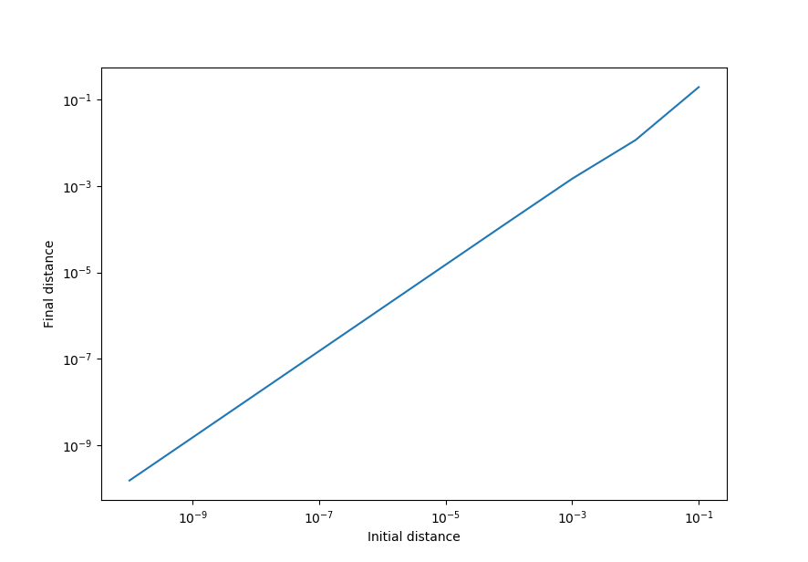
Thus the pendulum map is not sensitive to initial conditions for these values, implying periodicity (which we have already seen in the phase space diagrams above).

In contrast, the semicontinuous Clifford map for $a = -1.4, \; b = 1.7, \; c = 1.0, \; d = 0.7$ and $ \Delta t = 1.35$ (iterated for 500000 steps) is extremely sensitive to changes in initial values: going from $(x_0, y_0) = (10.75, 8.2)$ to $(x_0, y_0)= (10.750000001, 8.2)$ results in a significant change in final point location

p1 = (10.98448, 7.96167)
p2 = (11.03945, 8.26257)

If we shrink the distance between initial points to 0, the distance between final points does not decrease.

initial = 0.1    final = 3.775e-01
initial = 0.01    final = 3.060e-01
initial = 0.001    final = 3.097e-01
initial = 0.0001    final = 3.042e-01
initial = 1e-05    final = 4.195e-01
initial = 1e-06    final = 1.138e-01
initial = 1e-07    final = 4.368e-02
initial = 1e-08    final = 3.059e-01
initial = 1e-09    final = 3.143e-01
initial = 1e-10    final = 4.002e-01

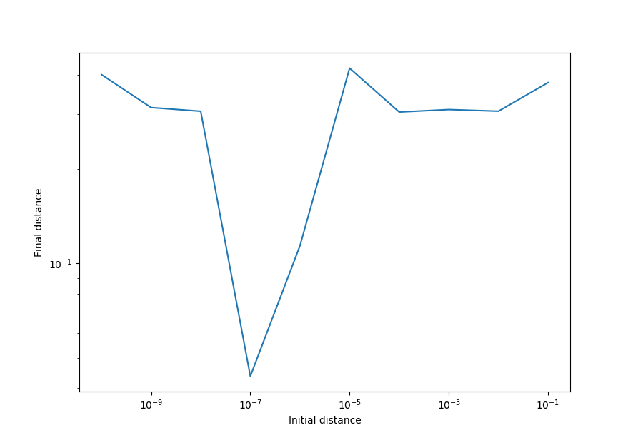
This means that the Clifford attractor is sensitive to initial values, implying that it is aperiodic for these parameters.

Pendulum map in the Clifford system

There are a number of similarities between widely different nonlinear systems. Perhaps the most dramatic example of this is the ubiquitous appearance of self-similar fractals in chaotic nonlinear systems. This may be most dramatically seen when the constant parameters of certain equation systems are tweaked such that the output produces a near-copy of another equation system, a phenomenon that is surprisingly common to nonlinear systems. For example, take the Clifford attractor:

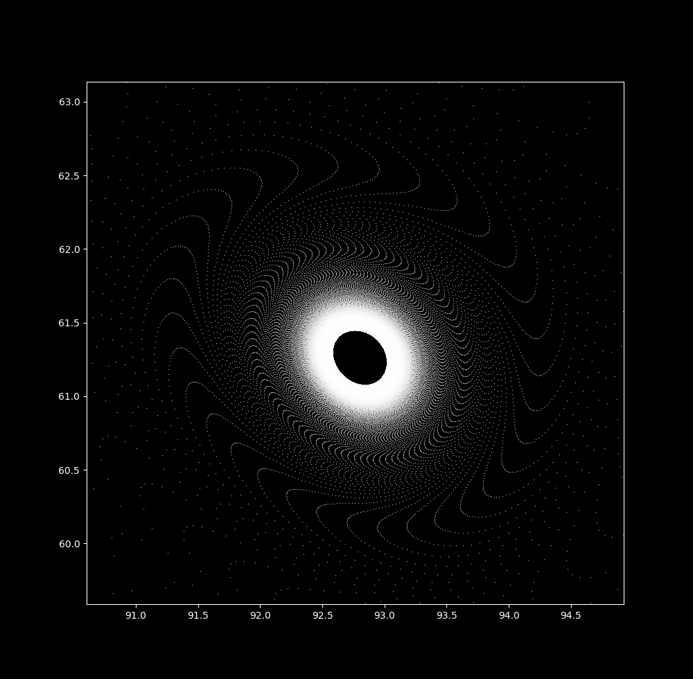
\[x_{n+1} = \sin(ay_n) + c \cdot \cos(ax_n) \\ y_{n+1} = \sin(bx_n) + d \cdot \cos(by_n) \tag{3}\]

This is clearly a very different system of equations than (1), and for most constant values it produces a variety of maps that look nothing like what is produced by the pendulum system. But observe what happens when we iterate semicontinuously (see here for more information), setting

\[a=-0.3, b=0.2, c=0.5, d=0.3, \Delta t = 0.9 \\ (x_0, y_0) = (90, 90)\]

We have a (slightly oblong) pendulum map!

---

If using large $\Delta t$ values yields a physically inaccurate map, what do these images mean?

There are some physically relevant reasons to increase a $\Delta t$ value:

1. The case of periodic forcing, where external energy is applied to a physical system in regular intervals. The dt value may be thought of as a direct measure of this energy, as a large enough $\Delta t$ will send this system towards infinity (ie infinite velocity).

2. When a field is intermittent: if a particle moves smoothly but only interacts with a field at regular time intervals, the same effect is produced.