Clifford attractor

Introduction

The Clifford attractor, also known as the fractal dream attractor, is the system of equations:

\[x_{n+1} = \sin( ay_n) + c \cdot \cos (ax_n) \\ y_{n+1} = \sin( bx_n) + d \cdot \cos (by_n) \tag{1}\label{eq1}\]

where a, b, c, and d are constants of choice. It is an attractor because at given values of a, b, c, and d, any starting point $(x_0, y_0)$ will wind up in the same pattern. See Vedran Sekara’s post for a good summary on how to use Python to make a plot of the Clifford attractor. Code for this page may be found here.

with $a = 2, b = 2, c = 1, d = -1$ the following map of \eqref{eq1} is made:

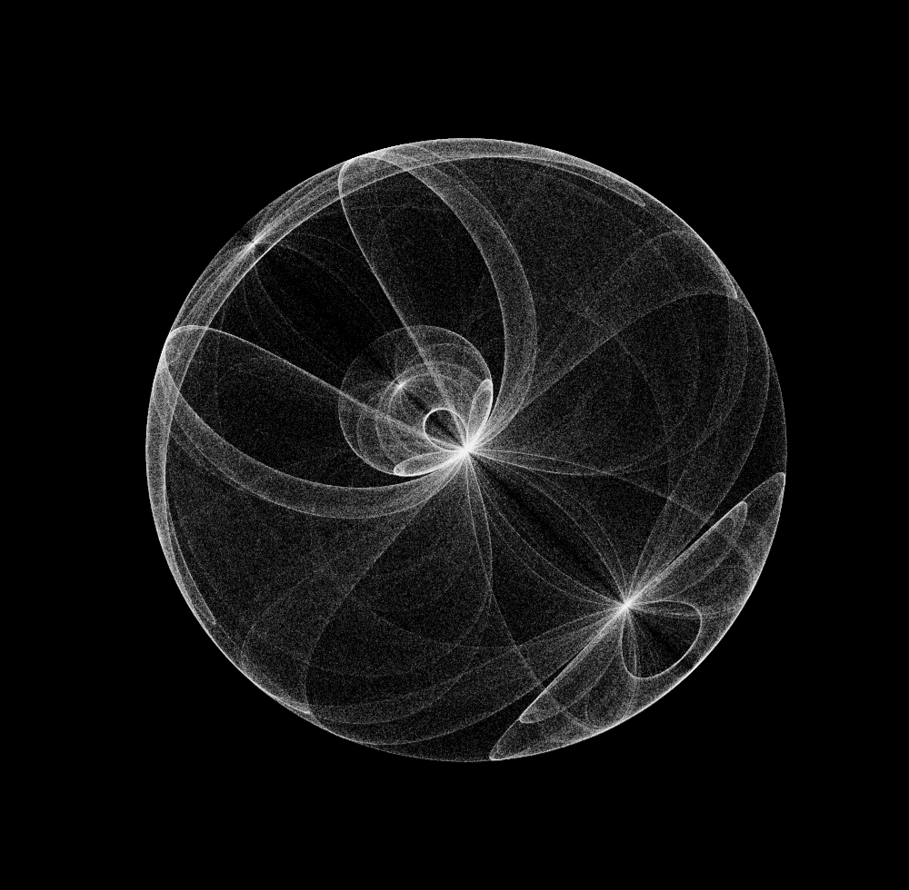
with $a = 2, b = 1, c = -0.5, d = -1.01$ ,

A wide array of shapes may be made by changing the constants, and the code to do this is here Try experimenting with different constants!

Clifford attractors are fractals

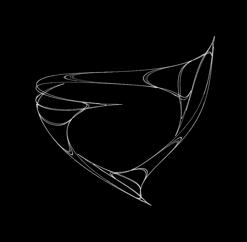
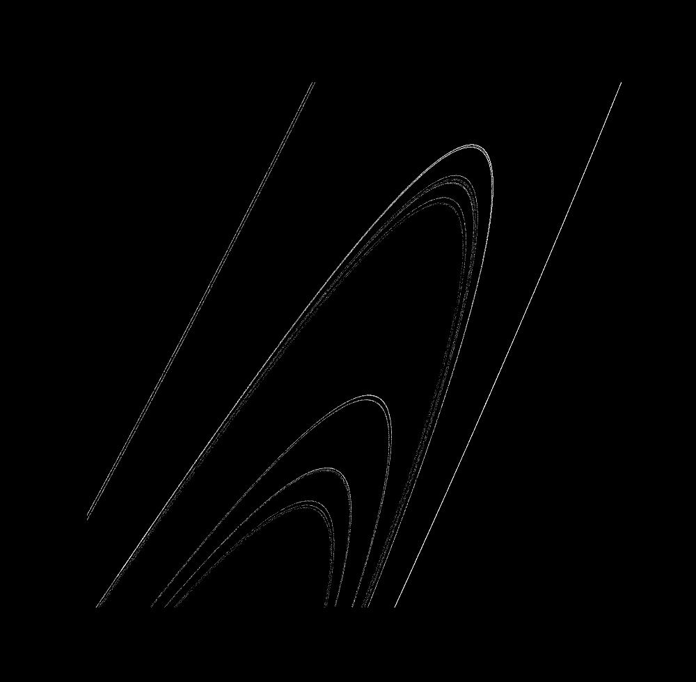
In what way is this a fractal? Let’s zoom in on the lower right side: In the central part that looks like Saturn’s rings, there appear to be 6 lines.

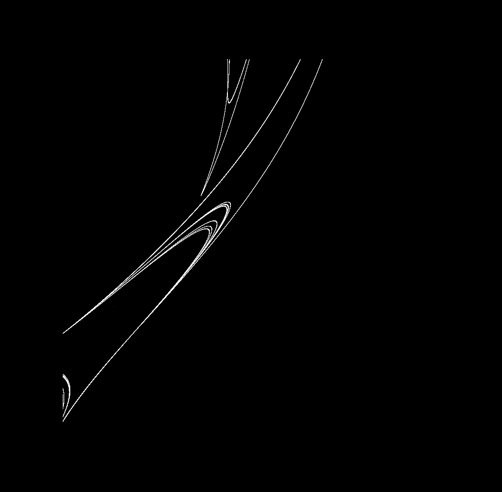
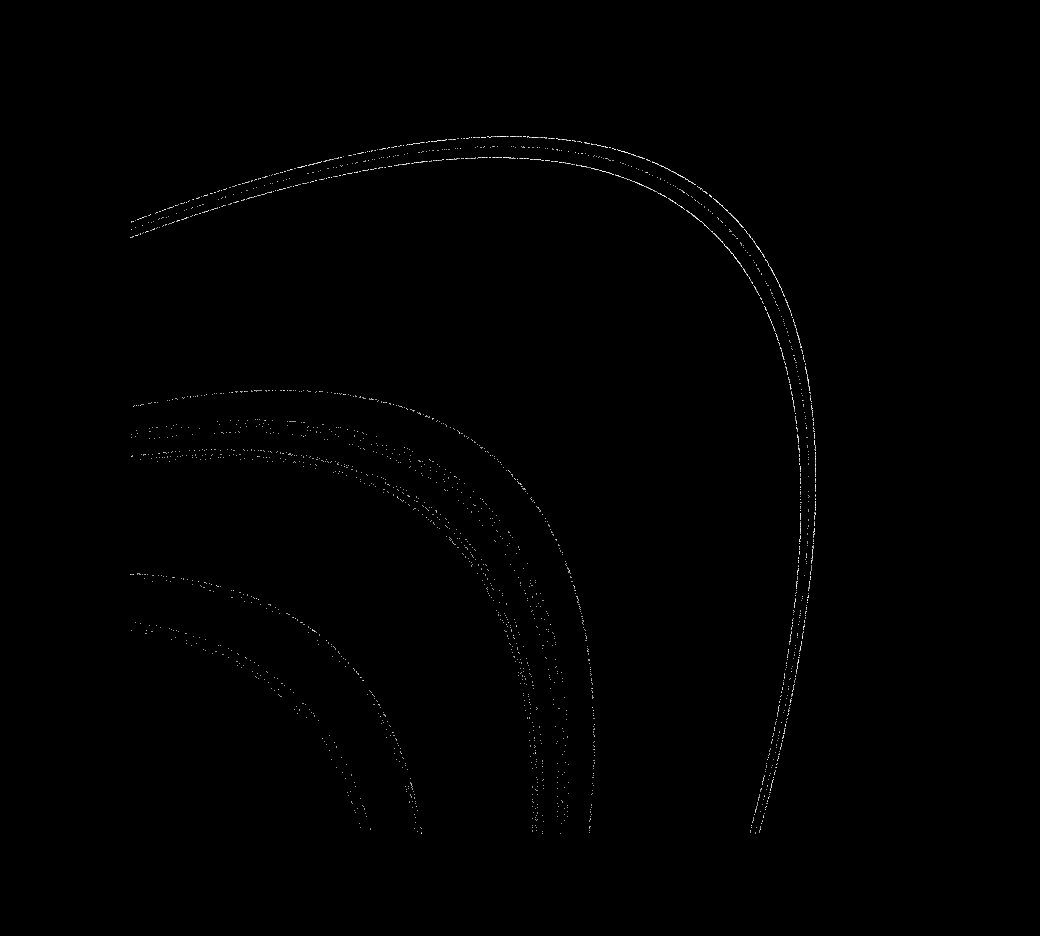
At a smaller scale, however, there are more visible, around 10

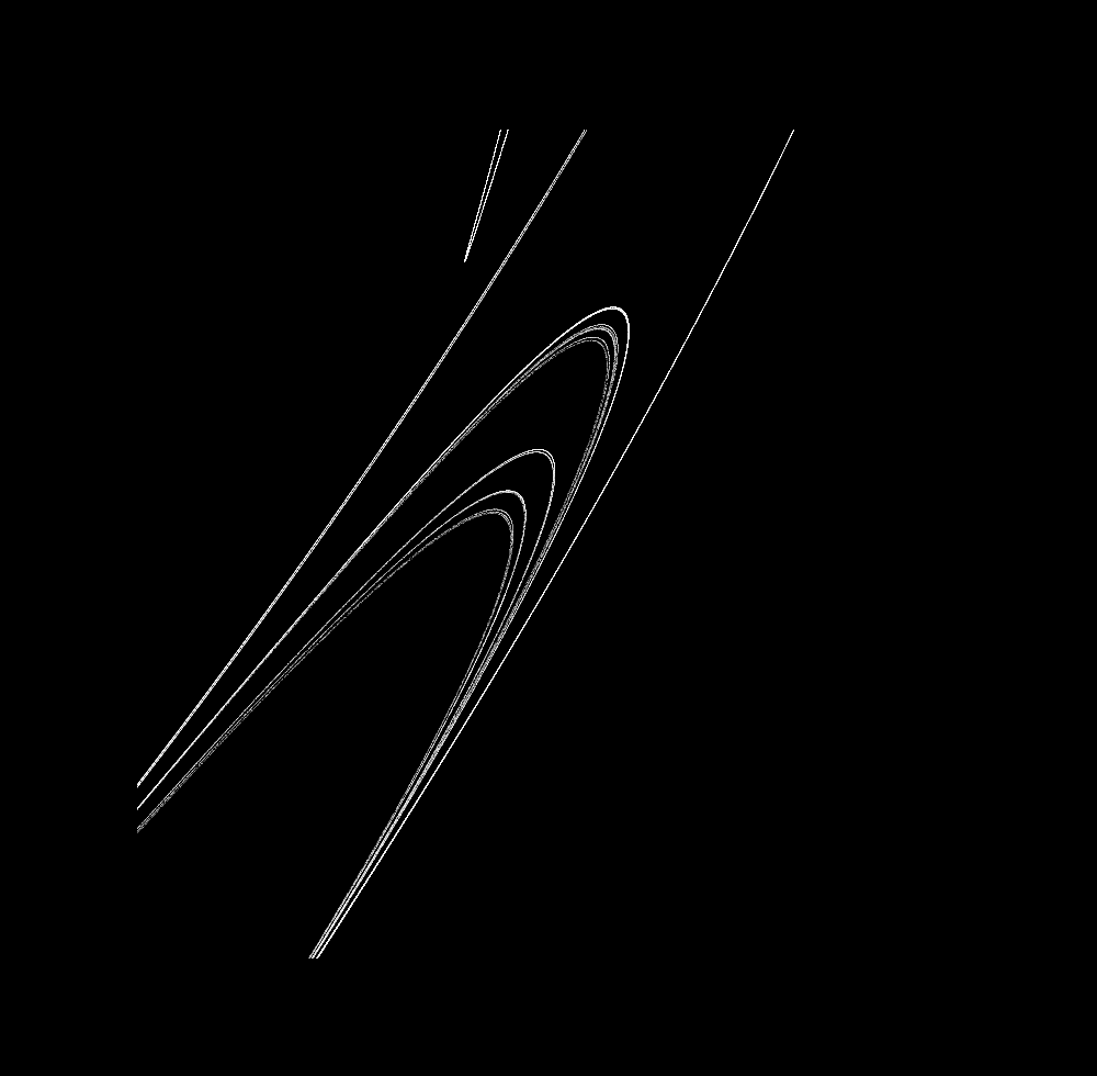
And at a smaller scale, still more,

and more at a smaller scale,

Fractals are objects that appear similar at different scale, or more precisely objects that have a scaling dimension greater than their topological dimension. In this case, we can idealize the topological dimension to be $d=1$, as after many iterations curves are formed. But upon an increase in scale, more and more lines within one boundary are visible: there are an infinite number of idealized curves that form a Cantor set, which has a scaling dimension greater than 0. For more on what fractals are and why they are important, see this page.

Clifford attractors shift dimension as constants change

For $a = 2.1, b = 0.8, c = -0.5, d = -1$, the attractor is three points:

For $b = 0.95$, more points:

For $b = 0.981$, the points being to connect to form line segments

And for $b = 0.9818$, a slightly-larger-than 1D attractor is produced

From $b=0.95$ to $b \approx 1.18$, incremented evenly:

The flashes are not a result of video artefacts, but instead represent small changes that lead to the attractor shifting back to points. Observe that the transition between a 0 and >1 dimensional attractor is not completely smooth! Small changes to $b$ lead to large changes in attractor dimension, even though the >1-dimensional attractor’s shape changes slowly.

This is not peculiar to the Clifford attractor: any one-to-one mapping from $1$ to $2$ dimensions must be discontinuous. And as there is no function that will map a point to a line (because any such function would have to map a point to many points, and would therefore not be a function), a vacuous observation is that there is no continuous mapping from 0 to 1 dimensions.

And when $b = 1.7$, a nearly-2d attractor is produced

Semi-continuous mapping

Say you want to model an ordinary differential equation:

\[\cfrac{dx}{dt} = f(x), \\\]

such that the change in the variable $x$ over time $t$ is defined by a function $f(x)$, starting at an initial point:

\[x(0) = x_0\]

ie the position of x at time 0 is some constant equal to $x_0$.

If the equation is nonlinear, chances are that there is no analytic solution. What is one to do? Do an approximation! Perhaps the simplest way of doing this is by using discrete approximations to estimate where a point will go given its current position and its derivative. This is known as Euler’s method, and can be expressed as follows:

\[x_{next} \approx x_{current} + \cfrac{dx_{current}}{dt} \cdot \Delta t\]

where $\cfrac{dx_{current}}{dt}$ signifies the differential equation evaluated at the current value of x.

With smaller and smaller values of $\Delta t$, the approximation becomes better and better but more and more computations are required for the same desired time interval:

\[x_{next} = x_{current} + \cfrac{dx_{current}}{dt} \cdot \Delta_t \quad as \, \Delta_t \to 0\]

For a two dimensional equation, the approximations can be made in each dimension:

\[\cfrac{dx}{dt} = sin(ay_n) + c \cdot cos(ax_n) \\ \cfrac{dy}{dt} = sin(bx_n) + d \cdot cos(by_n) \\ \\ x_{n+1} \approx x_n + \cfrac{dx}{dt} \cdot \Delta t \\ y_{n+1} \approx y_n + \cfrac{dy}{dt} \cdot \Delta t \tag{2}\]

To make these calculations and plot the results in python, the wonderful numpy and matplotlib libraries are used and we define the Clifford attractor function with constants $a=-1.4, \; b=1.7, \; c=1, \; d=0.7$:

# import third party libraries
import numpy as np 
import matplotlib.pyplot as plt 
plt.style.use('dark_background')

def clifford_attractor(x, y, a=-1.4, b=1.7, c=1.0, d=0.7):
	'''Returns the change in arguments x and y according to 
	the Clifford map equation. Kwargs a, b, c, and d are specified
	as constants.
	'''
	x_next = np.sin(a*y) + c*np.cos(a*x) 
	y_next = np.sin(b*x) + d*np.cos(b*y)
	return x_next, y_next

Setting up the number of iterations and the time step size, we then initialize the numpy array with 0s and add a starting $(x_0, y_0)$ coordinate:

# number of iterations
iterations = 1000000
delta_t = 0.01

# initialization
X = np.zeros(iterations)
Y = np.zeros(iterations)

# starting point
(X[0], Y[0]) = (10.75, 8.2)

For computing (2), let’s loop over the clifford function, adding in each next computed value to the numpy array.

# euler's method for tracking differential equations
for i in range(iterations-1):
	x_next, y_next = clifford_attractor(X[i], Y[i])
	X[i+1] = X[i] + x_next * delta_t
	Y[i+1] = Y[i] + y_next * delta_t

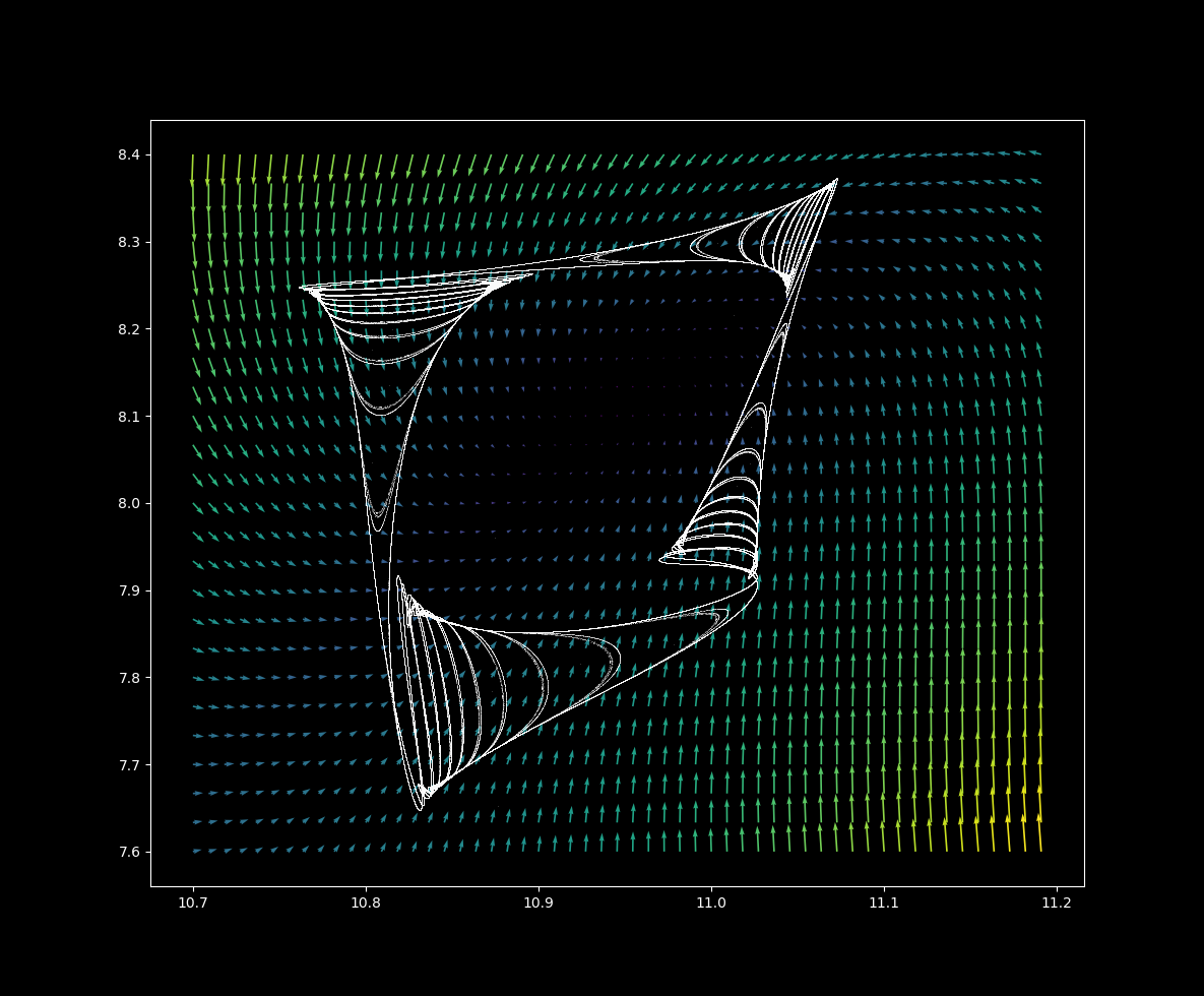
For continuous differential systems, one can follow a path along a vector grid in order to get an intuitive understanding of how the differential system influences a point’s path. To get a vector grid started, we define a grid using numpy with minimum, maximum, and intervals in the $(x,y)$ plane:

# Vector plot initialization
x = np.arange(10.7, 11.2, 1/110)
y = np.arange(7.6, 8.4, 1/30)

X2, Y2 = np.meshgrid(x, y)

The next step is to calculate the size and direction of each vector at the designated grid points according to the clifford map, and assign each value a color.

# calculate each vector's size and direction
a = -1.4
b = 1.7
c = 1.0
d = 0.7

dx = np.sin(a*Y2) + c*np.cos(a*X2)
dy = np.sin(b*X2) + d*np.cos(b*Y2)

color_array = (np.abs(dx) + np.abs(dy))**0.7

Now let’s plot the graph, adding both vector plot and differential iterations to the same plot.

# make and display figure
plt.figure(figsize=(10, 10))

# differential trajectory
plt.plot(X, Y, ',', color='white', alpha = 0.2, markersize = 0.05)

# vector plot
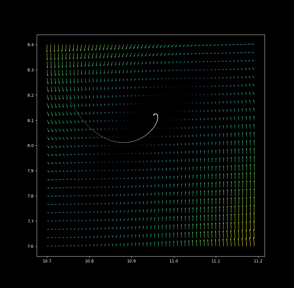
plt.quiver(X2, Y2, dx, dy, color_array, scale = 20, width=0.0018)
plt.axis('on')
plt.show()

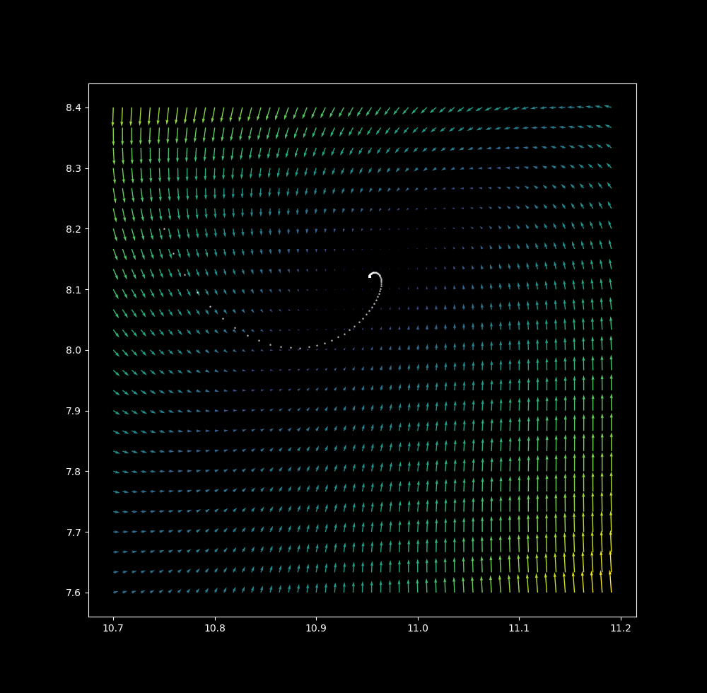
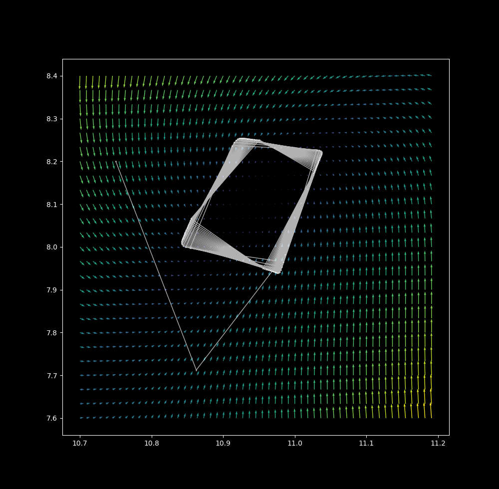
For a starting point situated at $ (x_0, y_0) = (10.75, 8.2)$, at $\Delta t = 0.01$ a smooth path along the vectors is made. The path is 1D, and the attractor is a point (which is zero dimensional).

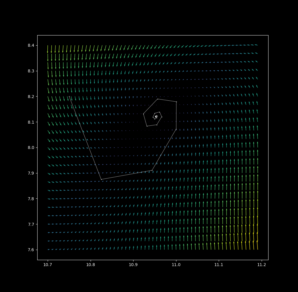
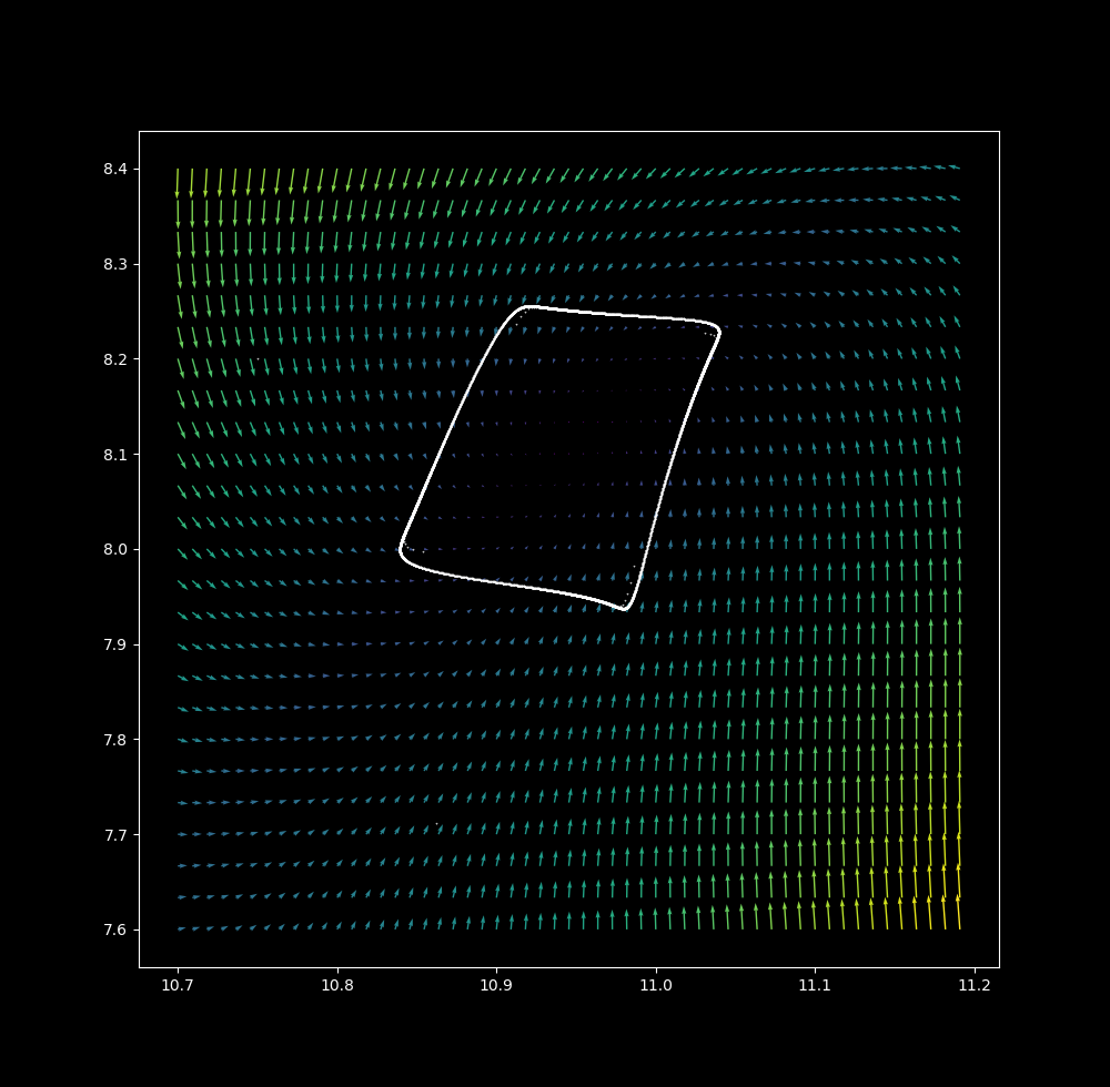
at $\Delta t = 0.1$

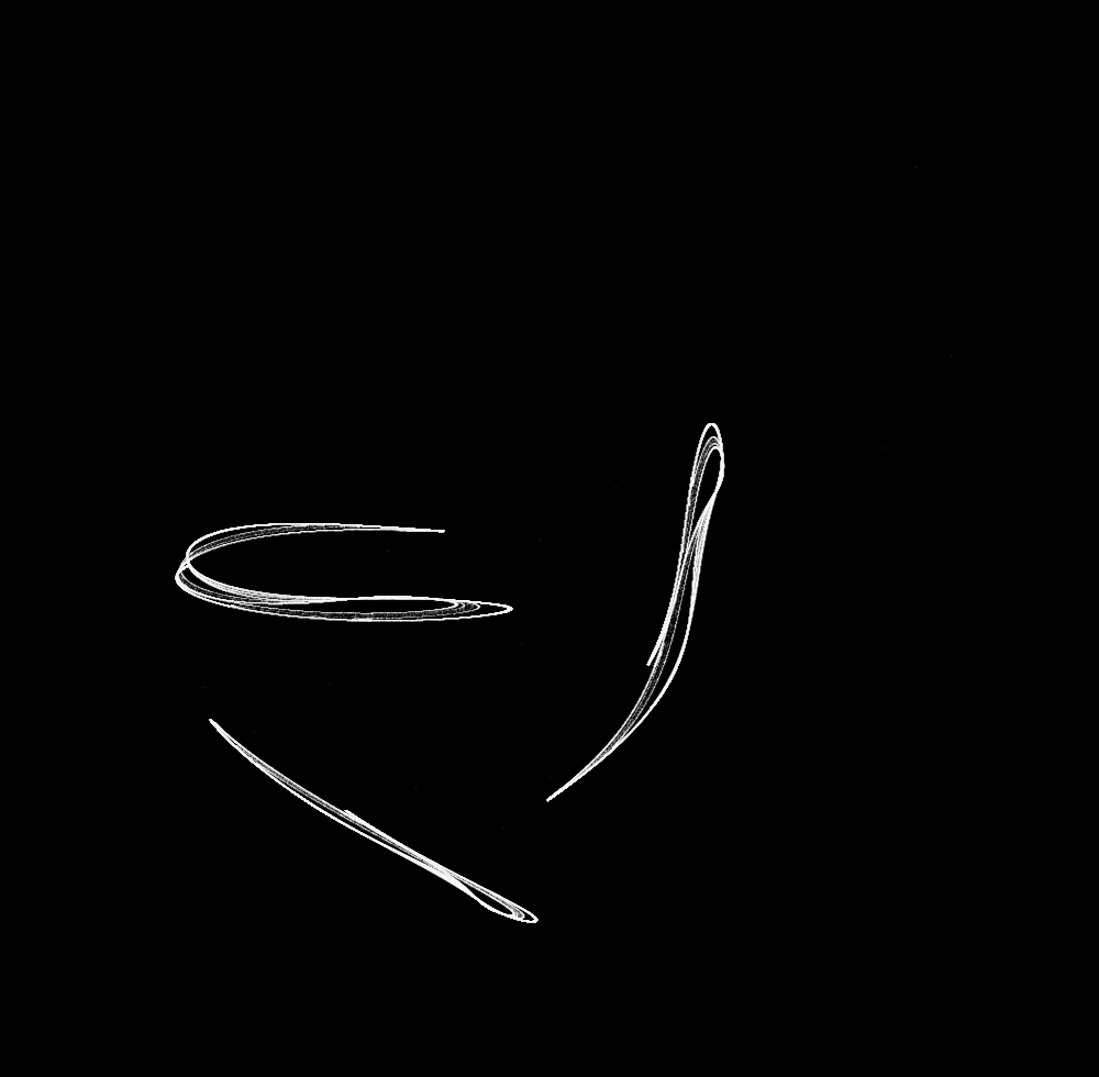
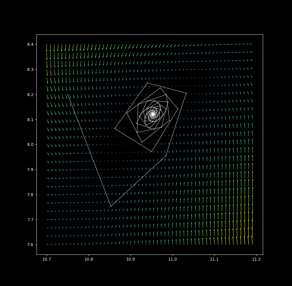
at $\Delta t = 0.8$ (points are connected for clarity)

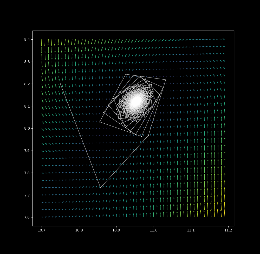
$\Delta t = 1.1$ the point attractor continues to unwind

$\Delta t = 1.15$

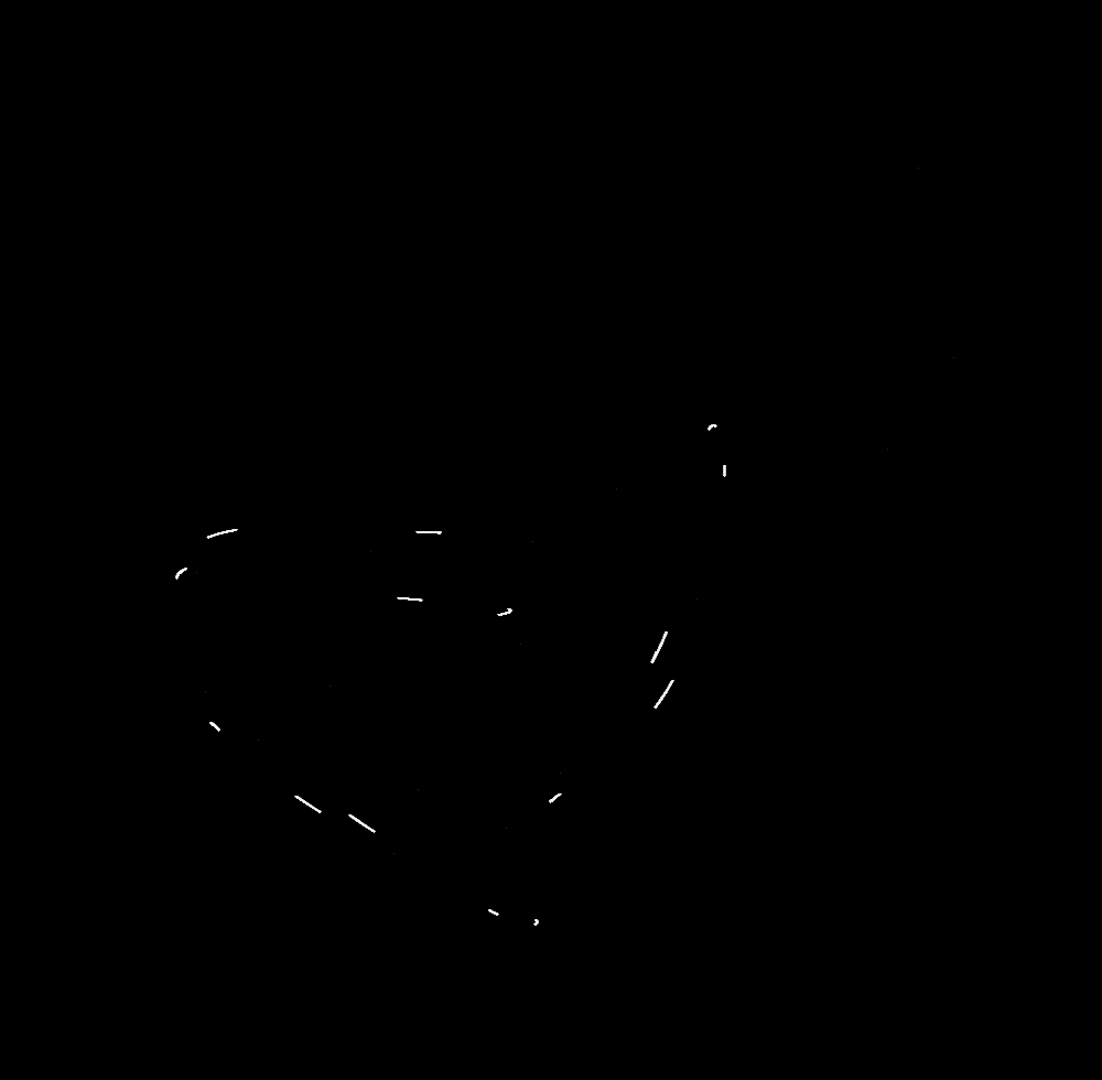
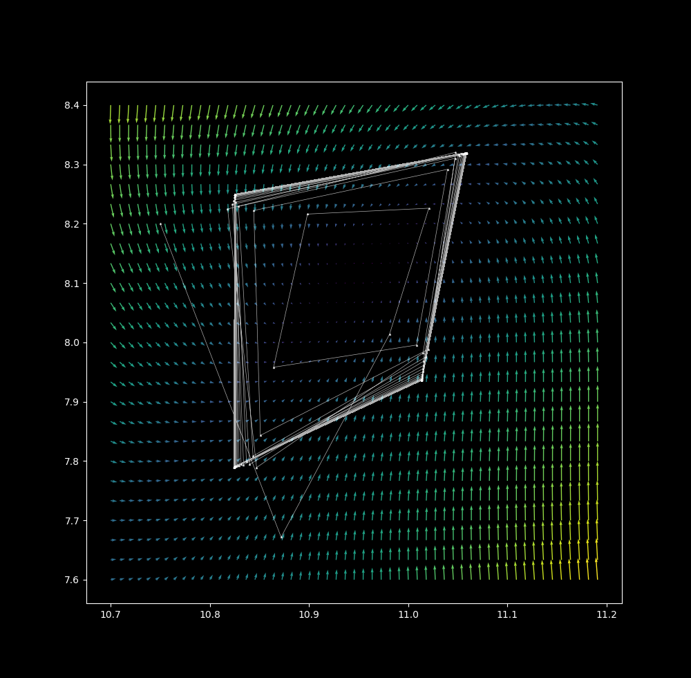
$\Delta t = 1.2$, the first few iterations reveal four slowly rotating lattice points

with more iterations at $\Delta t$ = 1.2, it is clear that the attractor is now 1 dimensional, and that the path is 0-dimensional. We have swapped a dimension in path for attractor!

$\Delta t = 1.3$ there are now 4 point attractors, and successive iterations come closer and closer to bouncing between these points.

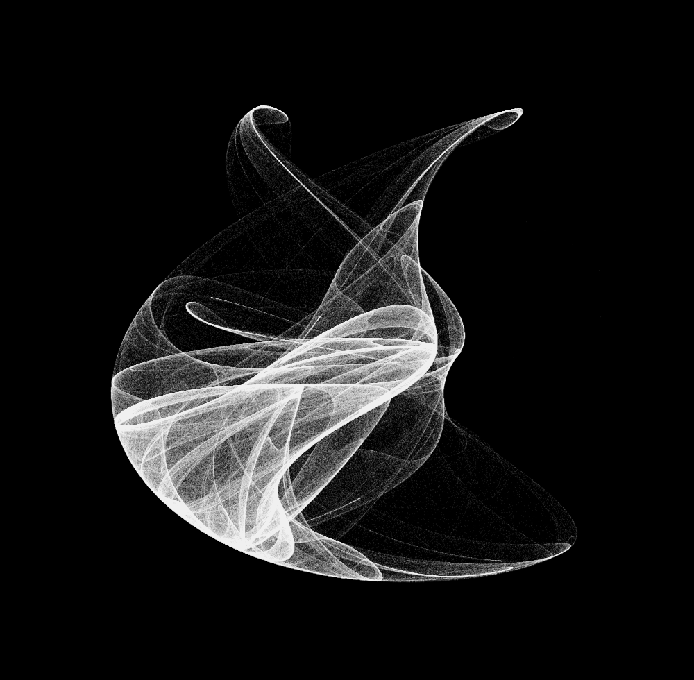
$\Delta t = 1.35$

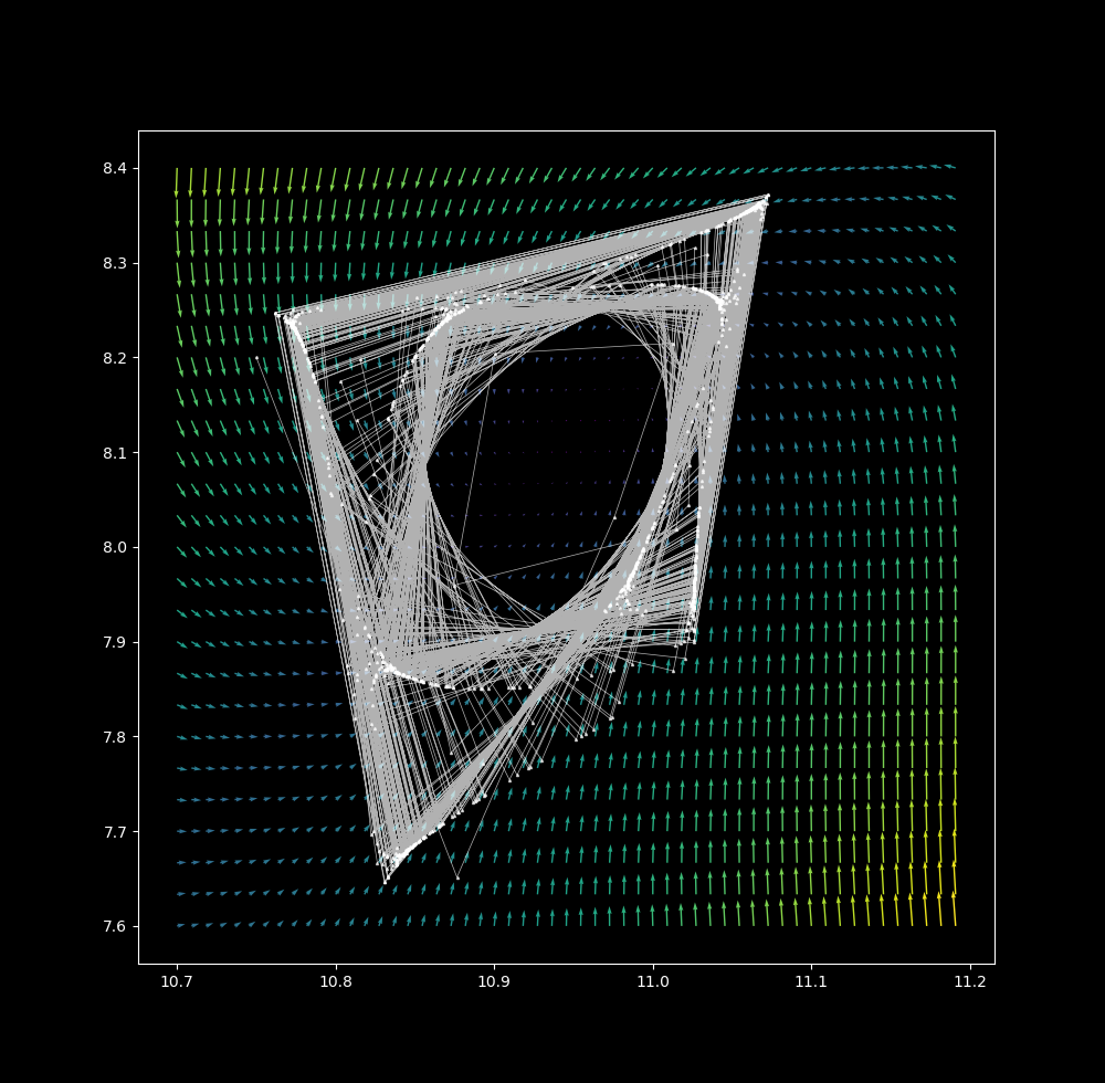
$\Delta t = 1.35$, a shape similar to the discrete map has formed.

From $\Delta t = 0.1 \to \Delta t = 1.35$,

For $\Delta t=1.35$, the final position after a sufficient number of iterations is extraordinarily sensitive to initial conditions, as detailed here. Sensitivity to initial values implies aperiodicity, and bounded aperiodic maps may contain fractals attractors (also called strange attractors.

Why semi-continuous?

Discrete differential systems are recurrence relations: a point’s next position is entirely determined by its current position according to the equation system given. In contrast, both a point’s next position in a continuous system is almost entirely determined by its current position: the equation system merely determines the direction and rate of change.

One can think of Euler maps with large $\Delta t$ values to be ‘semicontinuous’ because they represent amix between recurrence relations and (approximately) continuous maps: a point’s next position depends on both its current position as well as on the equation system’s output for that step.

Thus as is the case for continuous systems (and unlike that for discrete systems), one can trace a point’s path using a vector plot on a semicontinuous map. On the other hand, semi-continuous but not continuous maps of dissipative nonlinear equations may be fractals in two dimensions, as is the case for discrete maps (see here for an explanation).

Many attractors from one semi-continuous Clifford map

To generate a different Clifford attractor as defined in a discrete map, a change in the values of at least one of $a, b, c, d$ is required. But this is not the case for a semicontinuous map: merely by changing the starting $(x_0, y_0)$ coordinate, many (possibly infinitely many) attractors are possible.

For example, take the semicontinuous map with the same constants as before, $a=-1.4, \; b=1.7, \; c=1, \; d=0.7$ and with $\Delta t=1.35$. If the starting position is changed from $(x, y) = (10.75, 8.2)$ to $(x_0, y_0) = (25, 25)$, the following attractor is produced:

and at $(x_0, y_0) = (90, 90)$:

and as $\Delta t = 0.1 \to \Delta t = 1.35$ the attractor changes from point to line to fractal, but once again not smoothly:

The regions that attract all points into a certain attractor are called the basins of attraction (see the henon map page for more information). For example, the attractor (shown above) of the starting point $(x_0, y_0) = (10.75, 8.2)$ is also the attractor of the point $(x_0, y_0) = (10.5, 8)$ and the attractor of the point $(x_0, y_0) = (9, 7)$. Other starting points yield other attractors, so does steadily moving the starting point lead to smooth changes between attractors?

For $(x_0, y_0) = (7.5, 7.5) \to (x_0, y_0) \approx (12, 12)$, the transition from one basin of attraction to another is both abrupt and unpredictable: very small changes in starting position lead to total disappearence or change of the attractor for certain values. This causes the attractors to flash when $(x_0, y_0) = (7.5, 7.5) \to (x_0, y_0) \approx (12, 12)$

For an investigation into which point ends up where, see this page.