Image Classification with Convolutional Neural Networks

Introduction

In scientific research it is often important to be able to categorize samples accurately. With experience, the human eye is in many instances able to accurately discern and categorize many important features from microsopic observation.

Another way to accomplish this task is to employ a computational method. One could imagine attempting to program a machine to recognize the same features that an expert individual would take note of in order to replicate that individual’s performance. Historically this approach was taken in efforts resulting in what were called ‘expert systems’, but now such approaches are generally no longer attempted. This is for a couple reasons: firstly because they are extremely tedious and time-consuming to implement, and secondly because once implemented these methods generally fail to be very accurate. The underlying cause for both of these points of failure is that it is actually very difficult to explain complicated tasks like image recognition precisely yet generally enough to be accurate.

The failure of attempts to directly replicate complex tasks programatically has led to increased interest in the use of probability theory to make estimations rather than absolute statements, resulting in the expansion of a field of statistical learning. Particularly difficult tasks like image classification often require particularly detailed computational methods for best accuracy, and this computationally-focused statistical learning is called machine learning.

The current state-of-the-art method for classifying images via machine learning is achieved with neural networks. These are programs that use nodes called artificial ‘neurons’ that have associated weights and biases that are adjusted in accordance to some loss function in order to ‘learn’ during training. These neuron are arranged in sequential layers, each representing the input in a potentially more abstract manner before the output layer is used for classification. This sequential representation of the input in order to accomplish a machine learning task is the core idea behind the field of deep learning, encompasses artifical neural networks along with other models such as Boltzmann machines.

A hands-on introduction to the theory and utility of neural networks for image classification is found in Nielsen’s book, and the core algorithms of stochastic gradient descent and backpropegation that are used to train neural nets on this page are explained there. For a deeper and more comprehensive study of this and related topics, perhaps the best resource is the classic text by Goodfellow, Bengio, and Courville. This page will continue with the assumption of some familiarity with the fundamental ideas behind deep learning. Note thatexplanation of the utility of convolutions is given below, as this topic is particularly important to this page and is somewhat specialized to image-based deep learning models.

Neural networks are by no means simple constructions, but are not so prohibitively complicated that they cannot be constructed from scratch such that each operation to every individual neuron is clearly defined (see this repo for an example). But this approach is relatively slow: computing a tensor product element-wise in high-level programming languages (C, C++, Python etc) is much less efficient than computation with low-level array optimized libraries like BLAS and LAPACK. In python, numpy is perhaps the most well-known and powerful library for general matrix manipulation, and this library can be used to simplify and speed up neural network implementations, as seen here.

As effective as numpy is, it is not quite ideal for speedy computations with very large arrays, specifically because it does not optimize memory allocation and cannot make use of a GPU for many simultaneous calculations. To remedy this situation, there are a number of libraries were written for the purpose of rapid computations with the tensors, with Tensorflow and PyTorch being the most popular. Most of this page references code employing Tensorflow (with a Keras front end) and was inspired by the Keras introduction and load image tutorials.

Convolutions Explained

A convolution (in the context of image processing) is a function in which a pixel’s value is added to that of its neighbors according to some given weight. The set of weights are called the kernal or filter, and are usually denoted as $\omega$. Arguably the simplest example is the uniform kernal, which in 3x3 is as follows:

\[\omega = \frac{1}{9} \begin{bmatrix} 1 & 1 & 1 \\ 1 & 1 & 1 \\ 1 & 1 & 1 \\ \end{bmatrix}\]

To perform a convolution, this kernal is applied to each pixel in the input to produce an output image in which each pixel corresponds to the average of itself along with all adjacent pixels. To see how this kernal blurs an input, say the following pixel values were found somewhere in an image $f(x, y)$:

\[f(x, y) = \begin{bmatrix} 1 & 2 & 3 \\ 0 & 10 & 2 \\ 1 & 3 & 0 \\ \end{bmatrix}\]

The convolution operation applied to this center element of the original image $f(x_1, y_1)$ with pixel intensity $10$ now is

\[\omega * f(x_1, y_1) = \frac{1}{9} \begin{bmatrix} 1 & 1 & 1 \\ 1 & 1 & 1 \\ 1 & 1 & 1 \\ \end{bmatrix} * \begin{bmatrix} 1 & 2 & 3 \\ 0 & 10 & 2 \\ 1 & 3 & 0 \\ \end{bmatrix}\]

The two-dimensional convolution operation is computed in an analagous way to the one-dimensional vector dot (scalar) product. Indeed, the convolutional operation is what is called an inner product, which is a generalization of the dot product into two or more dimensions. Dot products convey information of both magnitude and the angle between vectors, and similarly inner products convey both a generalized magnitude and a kind of multi-dimensional angle between operands.

The calculation for the convolution is as follows:

\[\omega * f(x_1, y_1) = 1/9 (1 \cdot 1 + 1 \cdot 2 + 1 \cdot 3 + \\ 1 \cdot 0 + 1 \cdot 10 + 1 \cdot 2 + 1 \cdot 1 + 1 \cdot3 + 1 \cdot 0) \\ = 22/9 \\ \approx 2.44 < 10\]

so that the convolved output $f’(x, y)$ will have a value of $2.4$ in the same place as the unconvolved input $f(x, y)$ had value 10.

\[f'(x, y) = \begin{bmatrix} a_{1, 1} & a_{1, 2} & a_{1, 3} \\ a_{2, 1} & a_{2, 2} = 22/9 & a_{2, 3} \\ a_{3, 1} & a_{3, 2} & a_{3, 3} \\ \end{bmatrix}\]

Thus the pixel intensity of $f’(x, y)$ at position $m, n = 2, 2$ has been reduced. If we calculate the other values of $a$, we find that it is more similar to the values of the surrounding pixels compared to the as well. The full convolutional operation simply repeats this process for the rest of the pixels in the image to calculate $f’(x_1, y_1), …, f’(x_m, y_n)$. A convolution applied using this particular kernal is sometimes called a normalized box blur, and as the name suggests it blurs the input slightly.

But depending on the kernal, we can choose to not blur an image at all. Here is the identity kernal, which gives an output image that is identical with the input.

\[\omega = \begin{bmatrix} 0 & 0 & 0 \\ 0 & 1 & 0 \\ 0 & 0 & 0 \\ \end{bmatrix}\]

We can even sharpen an input, ie decrease the correlation between neighboring pixels, with the following kernal.

\[\omega = \begin{bmatrix} 0 & -1/2 & 0 \\ -1/2 & 2 & -1/2 \\ 0 & -1/2 & 0 \\ \end{bmatrix}\]

Why would convolutions be useful for deep learning models applied to images?

Feed-forward neural networks are composed of layers that sequentially represent the input in a better and better way until the final layer is able to perform some task. This sequential representation is learned by the model and not specified prior to training, allowing neural networks to accomplish an extremely wide array of possible tasks.

When passing information from one layer to the next, perhaps the simplest approach is to have each node (‘artificial neuron’) from the previous layer connect with each node in the next. This means that for one node in the second layer of width $n$, the activation $a_{m, n}$ is computed by adding all the weighted activations from the previous layer of width $m$ to the bias for that node $b_n$

\[a_{m, n} = \left( \sum_m w_m z_m \right ) + b_n\]

where $z_m$ is the result of a (usually nonlinear) function applied to the activation $a_m$ of the previous layer’s node to result in an output. The same function is then applied to $a_{m, n}$ to make the output for one neuron of the second layer, and the process is repeated for all node in layer $n$.

This is called a fully connected architecture, as each node from one layer is connected to all the nodes in the adjacent layers. For a two-layer network, it is apparent that the space complexity of this architecture with regards to storing the model’s parameters scales quadratically with $mn$, meaning that for even moderately sized inputs the number of parameters becomes extremely large if the second layer is not very small.

One approach to dealing with this issue is to simply not connect all the nodes from each layer to the next. If we use a convolution, we can learn only the parameters necessary to define that convolution, which can be a very small number (9 + 1 for a 3x3 kernal with a bias parameter). The weights learned for a kernal are not changed as the kernal is scanned accross the input image (or previous layer), although it is common practice to learn multiple kernals at once in order to allow more information to pass between layers.

The convolutional operation is slightly different when applied to inputs with many sub-layers, usually termed ‘features’. One example of this would be a natural image of 3 colors, each with its own sub-layer (R, G, B). It is standard practice to have each kernal learn a set of weights for each feature in the input, rather than share the weights for all features. Precisely, this means that for an image with three color channel and one output feature and a 3x3 kernal will learn $3 * 3 * 3$ weight and one bias parameters, which are used to calculate the output value

\[a_{m, n} = \sum_f \sum_k \sum_l w_{f, k, l} z_{f, m+k, n+l} + b_n\]

Each feature of the output learns a new kernal, meaning that for an input image with $3$ features $f_i$ and an output of $6$ features $f_o$ for the same kernal with $k$ parameters (here 3x3), there are $k * f_i * f_o = ( 3* 3) * 3* 6 = 162$ weight parameters in total. Note that the number of parameters required increases quadratically with the number of features in the input and output of the convolution, meaning that practical convolutional layers are limited in terms of how many features they can possibly learn.

Practicality aside, convolutions are very useful for image-based deep learning models. In this section, we have seen how different kernals are able to sharpen, blur, or else do nothing to an input image. This is not all: kernals can also transform an input to perform edge detection, texture filtering, and more. The ability of a neural network to learn the weights of a kernal allows it to learn which of these operations should be performed across the entire image.

Implementing a neural network to classify images

The first thing to do is to prepare the training and test datasets. Neural networks work best with large training sets composed of thousands of images, so we split up images of hundreds of cells into many smaller images of one or a few cells. We can also performed a series of rotations on these images: rotations and translation of images are commonly used to increase the size of the dataset of interest. These are both types of data augmentation, which is when some dataset is expanded by a defined procedure. Data augmentation should maintain all invariants in the original dataset in order to be representative of the information found there, and in this case we can perform arbitrary translations and rotations. But for other image sets, this is not true: for example, rotating a 6 by 180 degrees yields a 9 meaning that arbitrary rotation does not maintain the invariants of images of digits.

Code that implements this procedure is found here. Similar image preparation methods are also contained in Tensorflow’s preprocessing module.

Now let’s design the neural network architecture. We shall be using established libraries for this set, so reading the documentation for Keras and Tensorflow may be useful. First we write a docstring for our program stating its purpose and output, and import the relevant libraries.

# Standard library
from __future__ import absolute_import, division, print_function, unicode_literals
import os
import pathlib

# Third-party libraries
import tensorflow as tf
from tensorflow.keras import Model
from tensorflow.keras.layers import Dense, Conv2D, Flatten, Dropout, MaxPooling2D
from tensorflow.keras.preprocessing.image import ImageDataGenerator
from PIL import Image 
import numpy as np 
import matplotlib.pyplot as plt 

Now we can assign the directories storing the training and test datasets assembled above to variables that will be called later. Here data_dir is our training dataset and data_dir2 and data_dir3 are test datasets, which link to folders I have on my Desktop.

def data_import():
	"""
	Import images and convert to tensorflow.keras.preprocessing.image.ImageDataGenerator
	object

	Args:
		None

	Returns:
		train_data_gen1: ImageDataGenerator object of image for training the neural net
		test_data_gen1: ImageDataGenerator object of test images
		test_data_gen2: ImageDataGenerator object of test images
	"""

	data_dir = pathlib.Path('/home/bbadger/Desktop/neural_network_images',  fname='Combined')
	data_dir2 = pathlib.Path('/home/bbadger/Desktop/neural_network_images2', fname='Combined')
	data_dir3 = pathlib.Path('/home/bbadger/Desktop/neural_network_images3', fname='Combined')

Now comes a troubleshooting step. In both Ubuntu and MacOSX, pathlib.Path sometimes recognizes folders or files ending in ._.DS_Store or a variation on this pattern. These folders are empty and appear to be an artefact of using pathlib, as they are not present if the directory is listed in a terminal, and these interfere with proper classification by the neural network. To see if there are any of these phantom files,

	image_count = len(list(data_dir.glob('*/*.png')))

	CLASS_NAMES = np.array([item.name for item in data_dir.glob('*') 
				if item.name not in ['._.DS_Store', '._DS_Store', '.DS_Store']])

	print (CLASS_NAMES)
	print (image_count)

prints the number of files and the names of the folders in the data_dir directory of choice. If the number of files does not match what is observed by listing in terminal, or if there are any folders or files with the ._.DS_Store ending then one strategy is to simply copy all files of the relevant directory into a new folder and check again.

Now the images can be rescaled (if they haven’t been already), as all images will need to be the same size. Here all images are scaled to a heightxwidth of 256x256 pixels. Then a batch size is specified, which determines the number of images seen for each training epoch.

	### Rescale image bit depth to 8 (if image is 12 or 16 bits) and resize images to 256x256, if necessary
	image_generator = tf.keras.preprocessing.image.ImageDataGenerator(rescale=1./255)
	IMG_HEIGHT, IMG_WIDTH = 256, 256

	### Determine a batch size, ie the number of image per training epoch
	BATCH_SIZE = 400

From the training dataset images located in data_dir, a training dataset train_data_1 is made by calling image_generator on data_dir. The batch size specified above is entered, as well as the target_size and classes and subset kwargs. If shuffling is to be performed between epochs, shuffle is set to True.

image_generator also has kwargs to specify rotations and translations to expand the training dataset, although neither of these functions are used in this example because the dataset has already been expanded via rotations. The method returns a generator that can be iterated to obtain images of the dataset.

	train_data_gen1 = image_generator.flow_from_directory(
		directory=str(data_dir),
		batch_size=BATCH_SIZE, 
		shuffle=True, 
		target_size=(IMG_HEIGHT,IMG_WIDTH), 
		classes=list(CLASS_NAMES), 
		subset = 'training')

The same process is repeated for the other directories, which in this case contain test image datasets. An image set generation may be checked with a simple function that plots a subset of images. This is particularly useful when expanding the images using translations or rotations or other methods in the image_generator class, as one can view the images after modification.

train_data_gen1, test_data_gen1, test_data_gen2 = data_import()
image_batch, label_batch = next(train_data_gen1)

Assigning the pair of labels to each iterable in the relevant generators,

(x_train, y_train) = next(train_data_gen1)
(x_test1, y_test1) = next(test_data_gen1)
(x_test2, y_test2) = next(test_data_gen2)

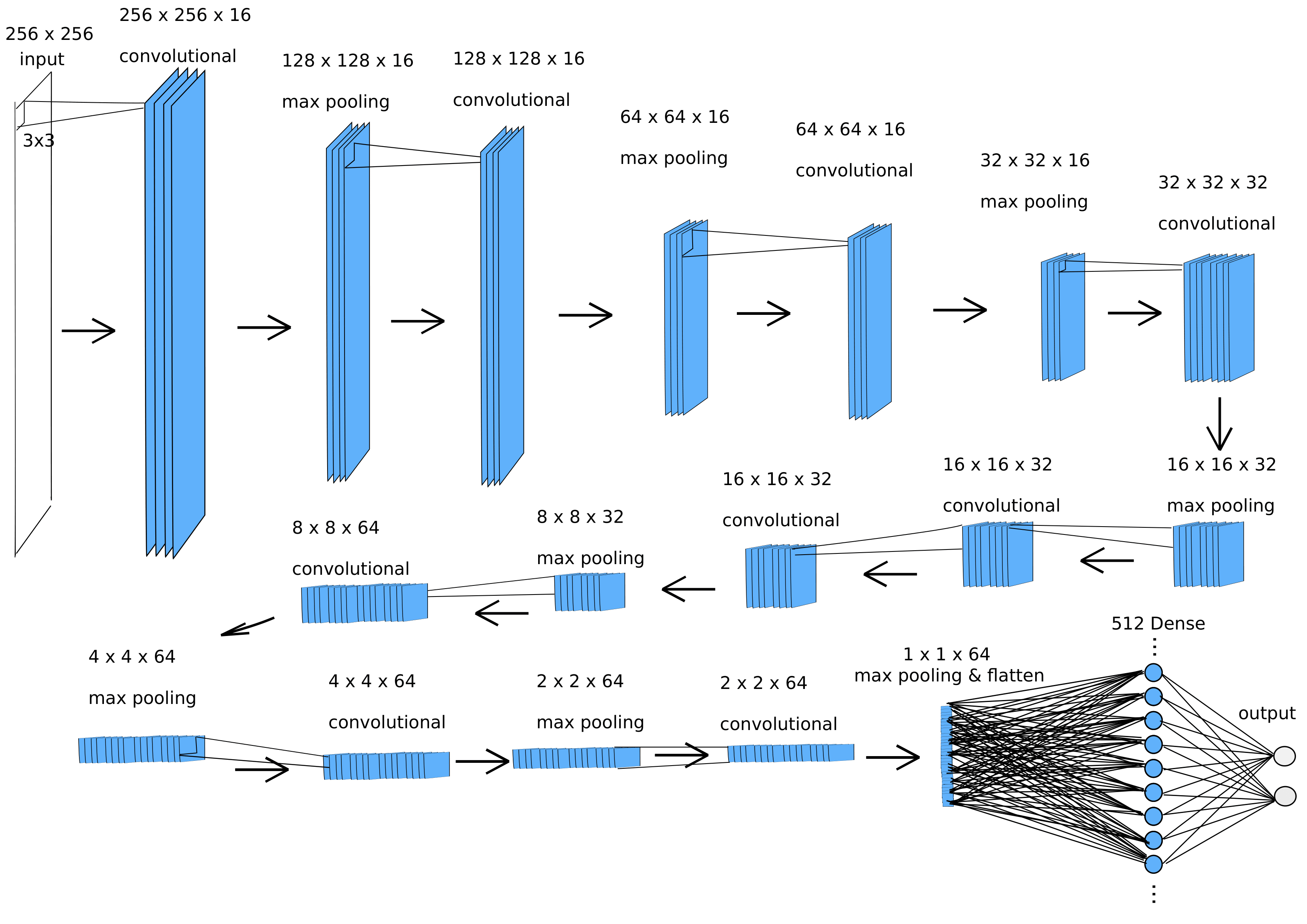
Now comes the fun part: assigning a network architecture! The Keras Sequential module is a straightforward, if relatively limited, class that allows a sequential series of network architectures to be added into one model. This does not allow for branching or recurrent architectures, in which case the more flexible functional Keras tensorflow.keras.Model should be used, and below is an example of the network implemented with this module. After some trial and error, the following architecture was found to be effective for the relatively noisy images here.

For any neural network applied to image data, the input shape must match the image x- and y- dimensions, and the output should be the same as the number of classification options. In this case, we are performing a binary classification between two cells, so the output layer of the neural network has 2 neurons and the input is specified by IMG_HEIGHT, IMG_WIDTH which in this case is defined above as 256x256.

The first step when using keras.Model is to create a class that inherits from keras.Model, and it is a good idea to inherit the objects of the parent class using super().__init__() as well

class DeepNetwork(Model):

    def __init__(self):
        super(DeepNetwork, self).__init__()
        self.entry_conv = Conv2D(16, (3, 3), padding='same', activation='relu', input_shape=(28, 28, 1), data_format='channels_last')
        self.conv16 = Conv2D(16, 3, padding='same', activation='relu')
        self.conv32 = Conv2D(32, 3, padding='same', activation='relu')
        self.conv32_2 = Conv2D(32, 3, padding='same', activation='relu')
        self.conv64 = Conv2D(64, 3, padding='same', activation='relu')
        self.conv64_2 = Conv2D(64, 3, padding='same', activation='relu')
        self.max_pooling = MaxPooling2D()

        self.flatten = Flatten()
        self.d1 = Dense(512, activation='relu')
        self.d2 = Dense(10, activation='softmax')
        

The way to read the Conv2D layer arguments is as follows: Conv2D(16, 3, padding='same', activation='relu') signifies 16 convolutional (aka filter) layers with a kernal size of 3, padded such that the x- and y-dimensions of each convolutional layer do not decrease, using ReLU (rectified linear units) as the neuronal activation function. The stride length is by default 1 unit in both x- and y-directions.

Now the class method call may be defined. This is a special method for classes that inherit from Module and is called every time an input is fed into the network and specifies way the layers initialized by __init__(self) are stitched together to make the whole network.

    def call(self, model_input):
        out = self.entry_conv(model_input)
        for _ in range(2):
            out = self.conv16(out)
            out = self.max_pooling(out)
	    
        out2 = self.conv32(out)
        out2 = self.max_pooling(out2)
        for _ in range(2):
            out2 = self.conv32_2(out2)
	    
        out3 = self.max_pooling(out2)
        out3 = self.conv64(out3)
        for _ in range(2):
            out3 = self.conv64_2(out3)
            out3 = self.max_pooling(out3)
	    
        output = self.flatten(out3)
        output = self.d1(output)
        final_output = self.d2(output)
	
        return final_output

The output being 10 neurons corresponding to 10 class types, which could be the genotypes of cells or some similar attribute.

Now the class DeepNetwork can be instantiated as the object model

model = DeepNetwork()

model is now a network architecture that may be represented graphically as

For optimal test classification accuracy at the expense of longer training times, an extra dense layer of 50 neurons was added to the above architecture. This may be accomplished by initializing self.d2 and adding this to call()

class DeepNetwork(Model):

    def __init__(self):
    ...
    
        self.d1 = Dense(512, activation='relu')
	self.d2 = Dense(50, activation='relu')
        self.d3 = Dense(10, activation='softmax')


	def call(self, model_input):
	...
	    output = self.flatten(out3)
	    output = self.d1(output)
	    output = self.d2(output)
	    final_output = self.d3(output)
	    return final_output
])

Now the network can be compiled, trained, and evaluated on the test datasets. model.summary() prints the parameters of each layer in our model for clarity.

model.compile(optimizer='Adam', 
	loss = 'categorical_crossentropy', 
	metrics=['accuracy'])

model.summary()
model.fit(x_train, y_train, epochs=9, batch_size = 20, verbose=2)
model.evaluate(x_test1, y_test1, verbose=1)
model.evaluate(x_test2, y_test2, verbose=1)

A few notes about this architecture: first, the output is a softmax layer and therefore yields a probability distribution for an easy-to-interpret result. The data labels are one-hot encoded, meaning that the label is denoted by a vector with one-hot tensor, ie instead of labels such as [3] we have [0, 0, 1]. In Tensorflow’s lexicon, categorical crossentropy should be used instead of sparse categorical crossentropy because of this.

Second, as there are only two categories used for the experiments below, the final layer was changed to have a 2-neuron output. Softmax was again used as the output activation function, which is not particularly advisable being that a 2-category softmax will tend to be unstable and result in high confidences for various predictions compared to the use of a sigmoid activation combined with a single-unit output (which is similar to a logistic regression for the final layer).

Softmax was retained in the final layer in the experiments below in order to purposefully add some instability to the final layer and force the network to choose between options confidently.

Accurate image classification

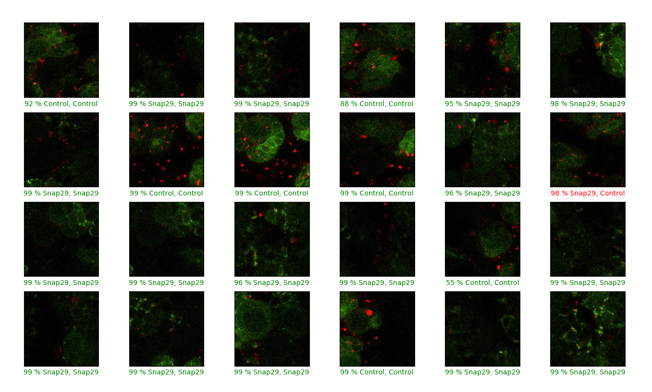
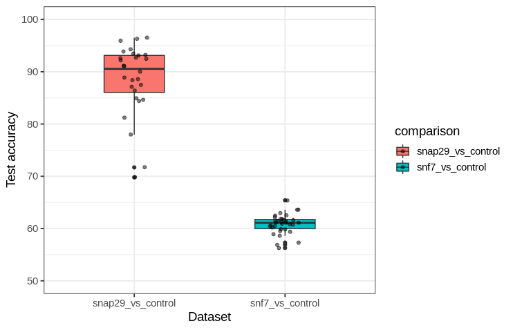
We follow a test/train split on this page: the model is trained on ~80% of the sample data and then tested on the remaining 20%, which allows us to estimate the model accuracy using data not exposed to the model during training. For reference, using a blinded approach by eye I classify 93 % of images correctly for certain dataset, which we can call ‘Snap29’ after the gene name of the protein that is depleted in the cells of half the dataset (termed ‘Snap29’) along with cells that do not have the protein depleted (‘Control’). There is a fairly consistent pattern in these images that differentiates ‘Control’ from ‘Snap29’ images: depletion leads to the formation of aggregates of fluorescent protein in ‘Snap29’ cells.

The network shown above averaged >90 % binary accuracy (over a dozen training runs) for this dataset. We can see these test images along with their predicted classification (‘Control’ or ‘Snap29’), the confidence the trained network ascribes to each prediction, and the correct or incorrect predictions labelled green or red, respectively. The confidence of assignment is the same as the activation of the neuron in the final layer representing each possibility.

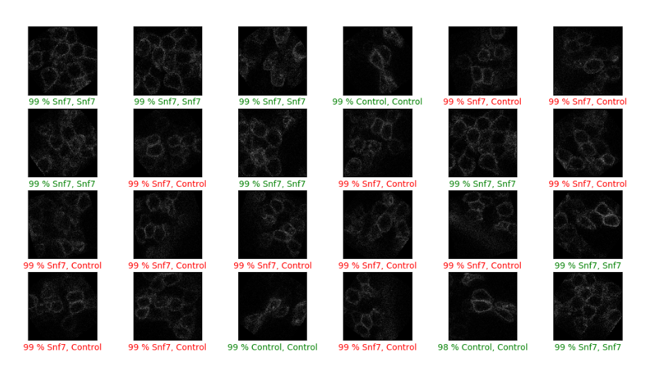
Let’s see what happens when the network is applied to an image set without a clear difference between the ‘Control’ and experimental group (this time ‘Snf7’, named after the protein depleted from these cells in this instance). After being blinded to the true classification labels, I correctly classified 71 % of images of this dataset. This is better than chance (50 % classification accuracy being that this is a balanced binary dataset) and how does the network compare? The average training run results in 62 % classification accuracy. We can see the results of one particular training run: the network confidently predicts the classification of nearly all images, but despite this confidence it is incorrect for many. Note that the confidence is a result of the use of softmax in the final layer.

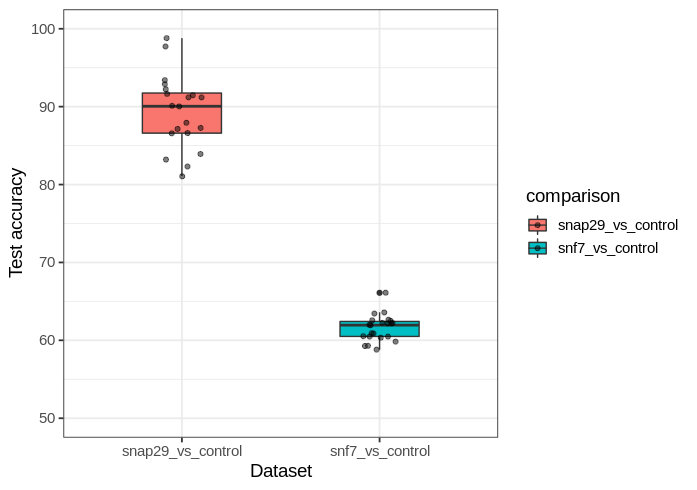
Each time a network is trained, there is variability in how effective the training is even with the same datasets as inputs. Because of this, it is helpful to observe a network’s performance over many training runs (each run starting with a naive network and ending with a trained one) The statistical language R (with ggplot) can be used to summarize data distributions, and here we compare the test accuracies of networks trained on the two datasets.

# R
library(ggplot2)

data1 = read.csv('~/Desktop/snf7_vs_snap29color_deep.csv')
attach(data1)
fix(data1)
l <- ggplot(data1, aes(comparison, test_accuracy, fill=comparison))
l + geom_boxplot(width=0.4) +
    geom_jitter(alpha=0.5, position=position_jitter(0.1)) +
    theme_bw(base_size=14) + 
    ylim(50, 100) +
    ylab('Test accuracy') +
    xlab('Dataset')
    

This yields

Generalization and training velocity

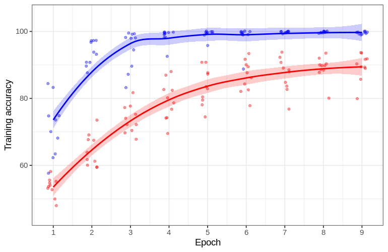
Why does the network confidently predict incorrect answers for the Snf7 dataset? Let’s see what happens during training. One way to gain insight into neural network training is to compare the accuracy of training image classification at the end of each epoch. This can be done in R as follows:

# R
library(ggplot2)
data7 = read.csv('~/Desktop/snf_training_deep.csv')
data6 = read.csv('~/Desktop/snap29_training_deep_2col.csv')

q <- ggplot() +
  # snf7
  geom_smooth(data=data7, aes(epoch, training.accuracy), fill='blue', col='blue', alpha=0.2) +
  geom_jitter(data=data7, aes(epoch, training.accuracy), col='blue', alpha=0.4, position=position_jitter(0.15)) +
  # snap29
  geom_smooth(data=data6, aes(epoch, training.accuracy), fill='red', col='red', alpha=0.2) +
  geom_jitter(data=data6, aes(epoch, training.accuracy), col='red', alpha=0.4, position=position_jitter(0.15))

q + 
  theme_bw(base_size=14) +
  ylab('Training accuracy') +
  xlab('Epoch') +
  ylim(50, 105) + 
  scale_x_continuous(breaks = seq(1, 9, by = 1))
  

As backpropegation lowers the cost function, we would expect for the classification accuracy to increase for each epoch trained. For the network trained on the Snap29 dataset, this is indeed the case: the average training accuracy increases in each epoch and reaches ~94 % after the last epoch. But something very different is observed for the network trained on Snf7 images: a rapid increase to 100 % training accuracy by the third epoch is observed.

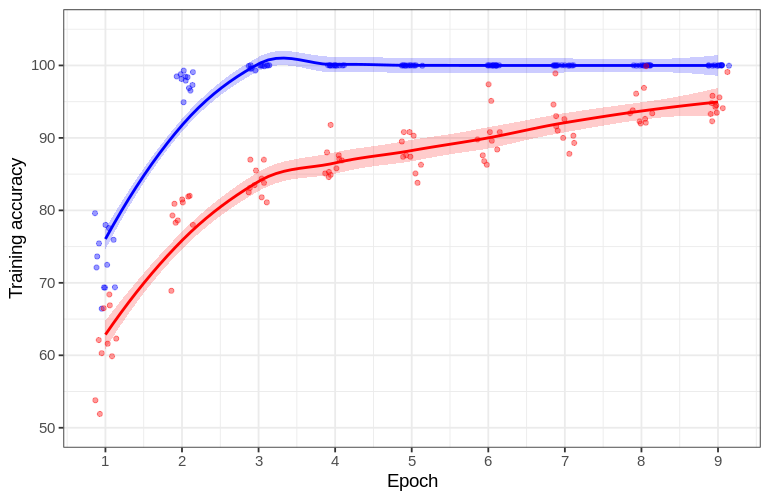
The high training accuracy (100%) but low test accuracy (62 %) for the network on Snf7 dataset images is indicative of a phenomenon in statistical learning called overfitting. Overfitting signifies that a statistical learning procedure is able to accurately fit the training data but fails to generalize previously-unseen test dataset. Statistical learning models (such as neural networks) with many degrees of freedom are somewhat prone to overfitting because small variations in the training data are able to be captured by the model regardless of whether or not they are important for true classification.

Overfitting is intuitively similar to memorization: both lead to an assimilation of information previously seen, without this assimilation necessarily helping the prediction power in the future. One can memorize exactly how letters look in a serif font, but without the ability to generalize then one would be unable to indentify many letters in a sans-serif font. The goal for statistical learning is to make predictions on hitherto unseen datasets, and thus to avoid memorization which does not guarantee this ability.

Thus the network overfits Snf7 images but is able to generalize for Snap29 images. This makes intuitive sense from the perspective of manual classification, as there is a relatively clear pattern that one can use to distinguish Snap29 images, but little pattern to identify Snf7 images.

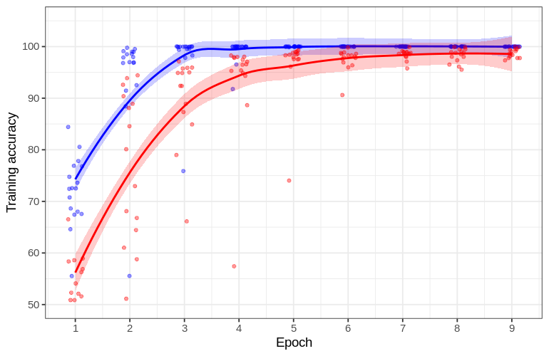
A slower learning process for generalization is observed compared to that which led to overfitting, but perhaps some other feature could be causing this delay in training accuracy. The datasets used are noticeably different: Snap29 is in two colors whereas Snf7 is monocolor. If a deeper network (with the extra layer of 50 dense neurons before the output layer) is trained on a monocolor version of the Snap29 or Snf7 datasets, the test accuracy achieved is nearly identical to what was found before,

And once again Snap29 training accuracy lags behind that of Snf7.

AlexNet revisited

To see if the faster increase in training accuracy for Snf7 was peculiar to the particular network architecture used, I implemented a model that mimics the groundbreaking architecture now known as AlexNet, and the code to do this may be found here. There are a couple differences between my recreation and the original that are worth mentioning: first, the original was split across two machines for training, leading to some parallelization that was not necessary for my training set. More substantially, AlexNet used a somewhat idiosyncratic normalization method that is related to but distinct from batch normalization, which has been substituted here.

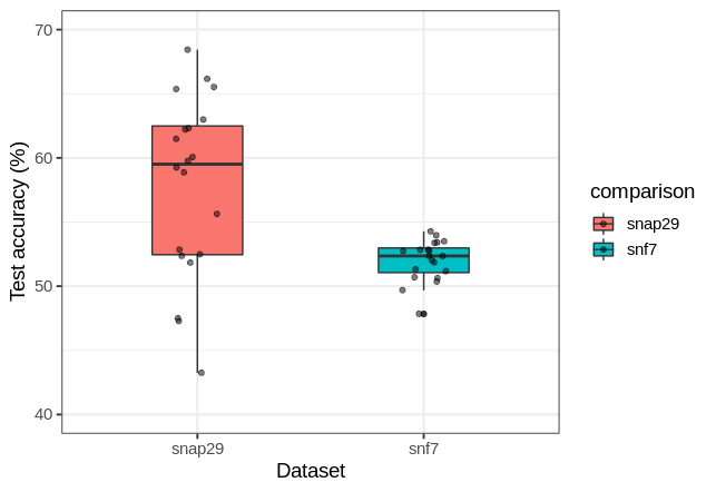
Using this network, it has previously been seen that overfitting is the result of slower increases in training accuracy relative to general learning (see this paper and another paper). With the AlexNet clone, once again the training accuracies for Snf7 increased faster than for Snap29 (although test accuracy was poorer for both relative to the deep network above). This suggests that faster training leading to overfitting in the Snf7 dataset is not peculiar to one particular network architecture and hyperparameter choice.

There are a number of interesting observations from this experiment. Firstly, the multiple normalization methods employed by AlexNet (relative to no normalization used for our custom architecture) are incapable of preventing severe overfitting for Snf7, or even for Snap29. Second, with no modification to hyperparameters the AlexNet architecture was able to make significant progress towards classifying Snap29 images, even though this image content is far different from the CIFAR datasets that AlexNet was designed to classify. The third observation is detailed in the next section.

How learning occurs

At first glance, the process of changing hundreds of thousands of parameters for a deep learning model seems to be quite mysterious. For a single layer it is perhaps simpler to understand how each component of the input influences the output such that the gradient of each component wrt. a function on the output may be computed, and once that is done the value of that parameter may be changed accordingly. But with many layers of input representation between the input and output, how does a gradient update to one layer not affect other layers? How accurate is gradient computation using backpropegation for deep learning models?

The answer to the latter question is that it is fairly accurate and not too difficult to compute the gradient itself, but the question of how the successive layers influence each other during gradient update is an outstanding one in the field of deep learning and has no clear answer as yet.

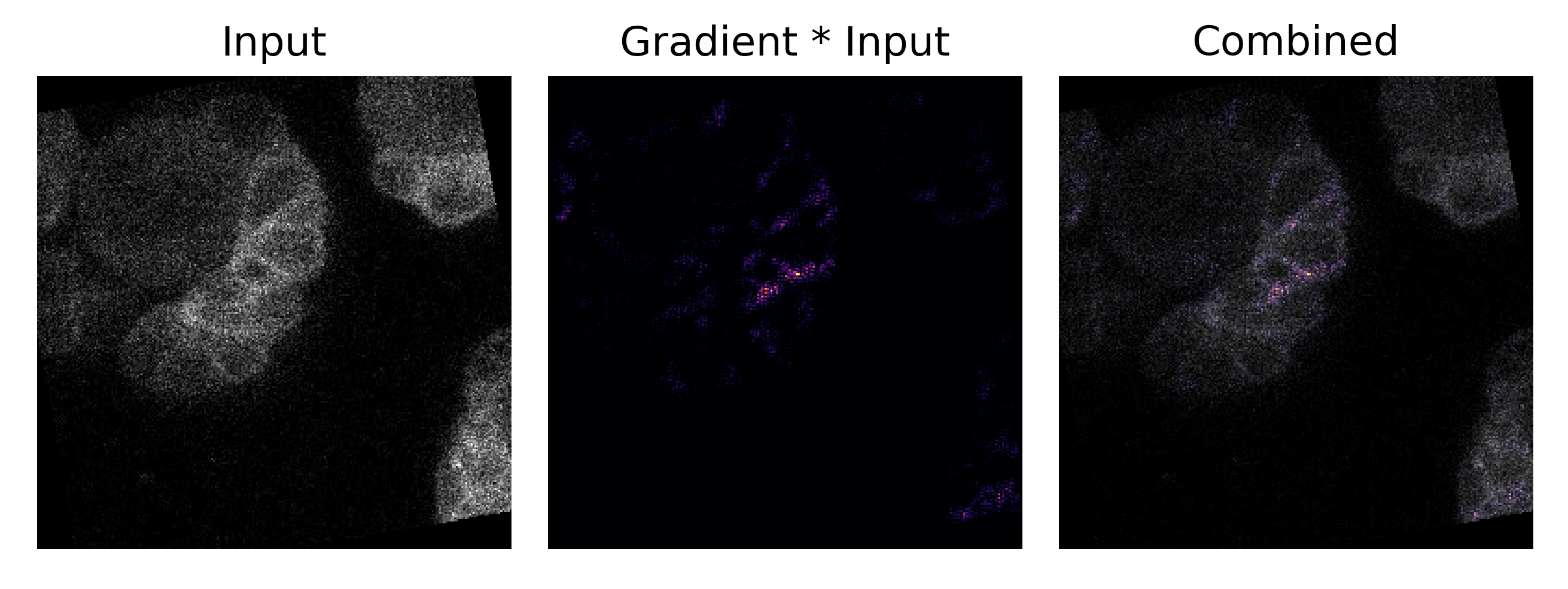
This does not mean that we cannot try to understand how learning occurs regardless. One way we can do this is to observe how the accuracy or model loss function changes over time as a model is fed certain inputs, and this is done in the preceding sections on this page. A more direct question may also be addressed: what does the model learn to ‘look at’ in the input?

We can define what a model ‘looks at’ most in the input as the inputs that change the output of the model the most, which is called input attribution. Attribution may be calculated in a variety of different ways, and here we will use a particularly intuitive method: gradient*input. The gradient of the output with respect to the input, projected onto the input, tells us how each input component changes when the output is moving in the direction of greatest ascent by definition. We simply multiply this gradient by the input itself to find how each input component influences the output. Navigate over to this page for a look at another attribution method and more detail behind how these are motivated.

Thus we are interested in the gradient of the model’s output with respect to the input multiplied by the input itself,

\[\nabla_a O(a; \theta) * a\]

where $\nabla_a$ is the gradient with respect to the input tensor (in this case a 1x256x256 monocolor image) and $O(a; \theta)$ is the output of our model with parameters $\theta$ and input $a$ and $*$ denotes Hadamard (element-wise) multiplication. This may be accomplished in Tensorflow as follows:

def gradientxinput(features, label):
	...
	optimizer = tf.keras.optimizers.Adam()
	features = features.reshape(1, 28, 28, 1)
	ogfeatures = features # original tensor
	features = tf.Variable(features, dtype=tf.float32)
	with tf.GradientTape() as tape:
		predictions = model(features)

	input_gradients = tape.gradient(predictions, features).numpy()
	input_gradients = input_gradients.reshape(28, 28)
	ogfeatures = ogfeatures.reshape(28, 28)
	gradxinput = tf.abs(input_gradients) * ogfeatures
	...

such that ogfeatures and gradxinput may be fed directly into matplotlib.pyplot.imshow() for viewing.

Earlier it was noted that a human may learn to distinguish between a healthy and unhealthy cell by looking for clumps of protein in the images provided. Does a neural network perform classification the same way? Applying our input attribution method to one particular example of an unhealthy cell image for a trained model, we have

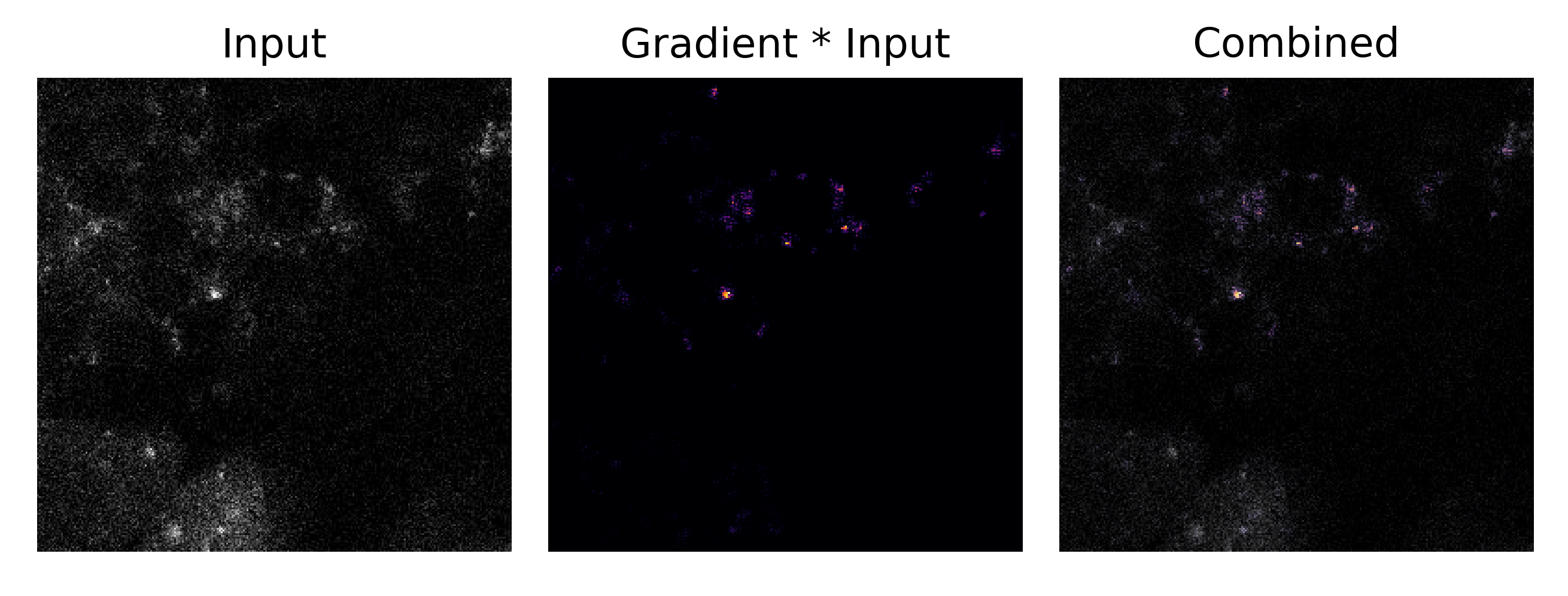
where the attributions are in purple and the original input image is in grayscale. Here it may clearly be seen that the clumps of protein overlap with the regions of highest attribution. It is interesting to note that the same attribution is applied to images of healthy cells:

Across many input images, a trained model tend to place the highest attribution on exactly these clumps accross many images (‘S’ denotes unhealthy and ‘C’ denotes healthy cells)

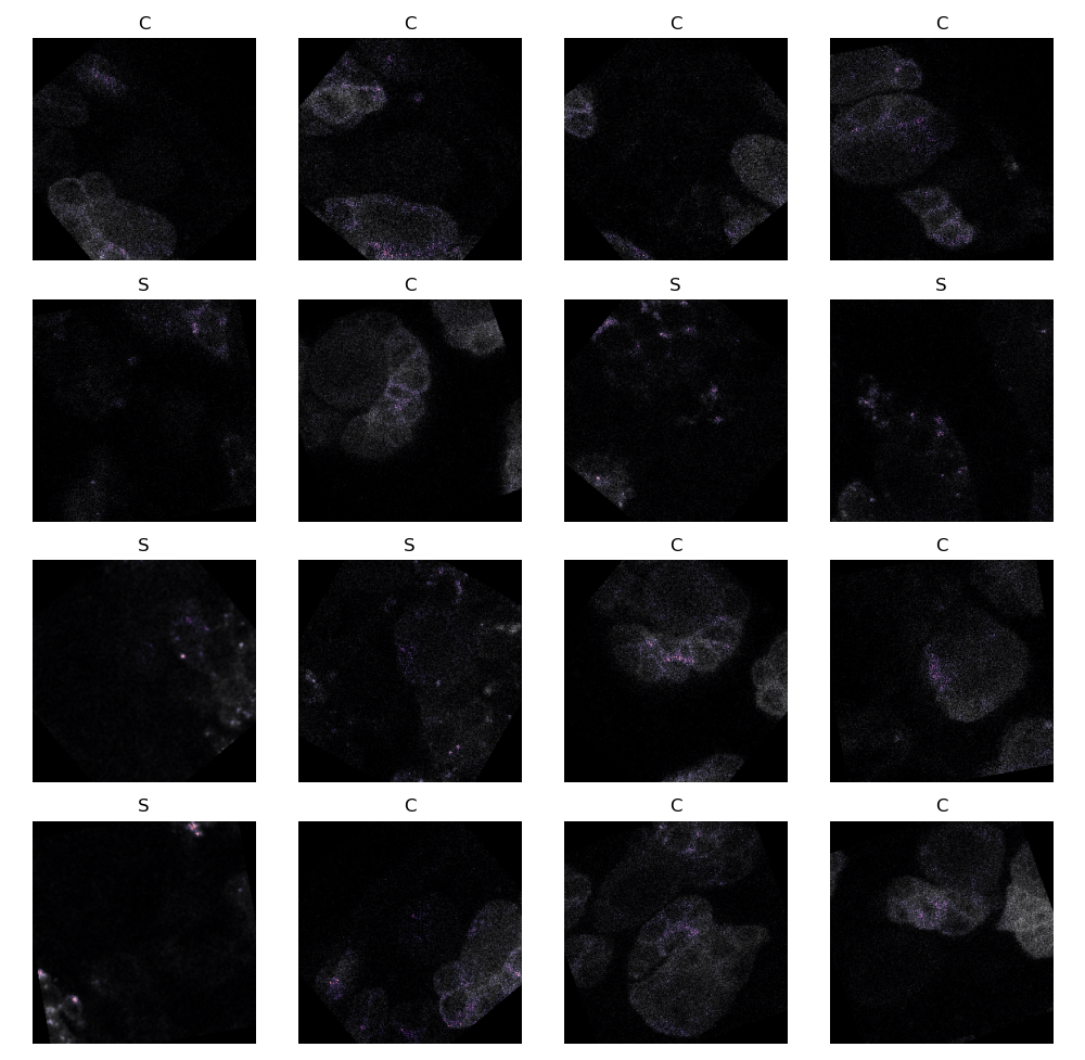
As a general rule, therefore, the deep learning models place the most importance on the same features as an expert human when attempting to classify the images of this particular set. The models effectively learn how to discriminate between classification options by determining how much of a clump of protein exists.

Learning does not equate to global minimization of a cost function during training

The above experimental results are quite interesting because they suggest that, for deep learning models of quite different architecture, a model’s ability to generalize depends not only on the model’s parameters $\theta$ and the family of functions that it can approximate given its possible outputs $O_n(\theta; a)$ but also on the choice of input $a$. Furthermore, the input $a$ is capable of inducing overfitting in a model employing extensive measures to prevent this phenomenon (L2 regularization, batch normalization) but a different input results in minimal overfitting (in the same epoch number) in a model that has none of these measures (nor any other regularizers separate from the model architecture itself).

Why is this the input so important to the behavior of the network? Neural networks learn by adjusting the weights and biases of the neurons in order to miminize a cost function, which is a continuous and differentiable representation of the accuracy of the output of the network. This is usually done with a variant on stochastic gradient descent, which involves calculating the gradient (direction of largest change) using a randomly chosen subset of images (which is why it is ‘stochastic’). This is conceptually similar to rolling a ball representing the network down a surface representing the multidimensional weights and biases of the neurons. The height of the ball represents the cost function, so the goal is to roll it to the lowest spot during training.

As we have seen in the case for Snf7 dataset images, this idea is accurate for increases in training accuracy but not not necessarily for general learning: reaching a global minimum for the cost function (100 % accuracy, corresponding to a cost function of less than 1E-4) led to severe overfitting and confident prediction of incorrect classifications. This phenomenon of overfitting stemming from a global minimum in the cost function during training is not peculiar to this dataset either, as it has also been observed elsewhere.

If decreasing the neural network cost function is the goal of training, why would an ideal cost function decrease (to a global minimum) not be desirable? In our analogy of a ball rolling down the hill, something important is left out: the landscape changes after every minibatch (more accurately, after every computation of gradient descent and change to neuronal weights and biases using backpropegation). Thus as the ball rolls, the landscape changes, and this change depends on where the ball rolls.

In more precise terms, for any given fixed neural network or similar deep learning approach we can fix the model architecture to include some set of parameters that we change using stochastic gradient descent to minimize some objective function. The ‘height’ $l$ of our landscape is the value of the objective function, $J$.

In this idealized scenario, the objective function $J$ is evaluated on an infinite number of input examples, but practically we can only evaluate it on a finite number of training examples. The output $O$ evaluated on set $a$ of training examples parametrized by weights and biases $\theta$ is $O(a; \theta)$ such that the loss function given true output $y$ is

\[l = J(O(a; \theta), y)\]

What is important to recognize is that, in a non-idealized scenario, $l$ can take on many different values for any given model configuration $\theta$ depending on the specific training examples $a$ used to evaluate the objective function $J$. Thus the ‘landscape’ of $h$ changes depending on the order and identity of inputs $a$ fed to the model during training, even for a model of fixed architecture. This is true for both the frequentist statistical approach in which there is some single optimal value of $\theta$ that minimizes $h$ as well as the Bayesian statistical approach in which the optimal value of $\theta$ is a random variable as it is unkown whereas any estimate of $\theta$ using the data is fixed.

As $j$ is finite, an optimal value (a global minimum) of $h$ can be achieved by using stochastic gradient descent without any form of regularization, provided that the model has the capacity to ‘memorize’ the inputs $a$. This is called overfitting, and is strenuously avoided in practice because reaching this global minimum nearly always results in a model that performs poorly on data not seen during training. But it is important to note that this process of overfitting is indeed identical to the process of finding a global (or asymptotically global) minimum of $l$, and therefore we can also say that regularized models tend to actually effectively avoid configurations $\theta$ that lead to absolute minima of $l$ for a given input set $a$ and objective function $J$.