Interpretable Deep Learning

Introduction

This page is part II in a series, for part I see this page.

It has been claimed in the past that deep learning is somewhat of a ‘black box’ machine learning approach: powerful, but mysterious with respect to understanding how a model arrived at a prediction. For a clear example of a machine learning technique that is the opposite of this, let’s revisit the linear regression.

\[\hat {y} = w^Tx + b \tag{1}\]

In some respect, training this approach is similar to training a neural network: the weight $w$ bias $b$ vectors are adjusted in order to minimize a cost function. Note that although we could train a linear regression model with gradient descent, it is more efficient to note that the gradient of the cost function in quadratic and therefore simply finding the point with 0 gradient algebraically allows us to minimize the cost function in one step.

Linear regression is, as the name implies, linear with respect to the parameters that we train. This means that for the regression function $f$, all parameters $w_n \in {w}$ and $b_n \in {b}$ are additive

\[f(w_1 + w_2) = f(w_1) + f(w_2) \\\]

and scaling

\[f(a*w_1) = a*f(w_1)\]

which is why the model is simple to optimize (as the gradient of this model is quadratic, and thus has one extremal point that can be found via direct computation of where $\nabla_w w^Tx + b = 0$ and $\nabla_b w^Tx + b = 0$.

But most importantly for transparency, this means that there are clear interpretations of any linear model. Say we have a regression that has 10 variables and the model assigns a weight of 0.1 to the first variable, and 2.5 to the second. From only this information, we know that the same change in the second variable as the first will lead to a 25-times increase in the response prediction. This follows directly from the additive (which means that we can consider each parameter separately) and scaling (such that constant terms may be taken outside a function mapping) nature of linear functions.

Say one were trying to predict how many rubber duckies were in a pool, and this prediction depended on 10 variables, the first two being how many rubber duck factories were nearby and the second how many people at the pool who like rubber ducks. If the second variable has a larger weight than the first, it is more important for predicting the output. We can even say that for every person who brings a rubber duck, we will have 2.5 more ducks in the pool.

This contrived example is to illustrate the very natural way that linear models may be interpreted: they key idea here is that one can separate out information for each input because the model itself is additive, and furthermore that we can know what the model will predict when we change a variable because all linear models are scaling.

Nonlinear models may be non-additive, non-scaling, or both non-additive and non-scaling. In our above example, this could mean that we have to examine all 10 variables at once to make any prediction, and furthermore that we have to know how many rubber ducks are in the pool to make a prediction of how many will be added by changing any of the variables.

Thus nonlinear models by their nature are not suited for interpretations that assume linearity. But we may still learn a great deal about how they arrive at the outputs they generate if we allow ourselves to explore further afield than linear interpretations. One widely used class of method to interpret nonlinear models is called attribution, and it involves determining the most- and least-important parts of any given input.

Attribution via Occlusion

Given any nonlinear model that performs a function approximation from inputs to outputs, how can we determine which part of the input is most ‘important’? Importance is not really a mathematical idea, and is too vague a notion to proceed with. Instead, we could say that more important inputs are those for which the output would be substantially different if those particular inputs were missing, and vice versa for less important inputs.

This definition leads to a straightforward and natural method of model interpretation that we can apply to virtually any machine learning approach. This is simply to first compute the output for some input, and then compare this output to a modified output that results from removing elements of the input one by one. This technique is sometimes called a perturbation-style input attribution, because we are actively perturbing the input in order to observe the change in the output. More commonly this method is known as ‘occlusion’, as it is similar to the process of a non-transparent object occluding (shading) light on some target.

There are a few different ways one can proceed with implementing occlusion. For a complete input map $x_c$ and a map of an input missing the first value ($x_i$),

\[x_c = f(1 \; 2015-02-06 \; 22:24:17 \;1845 \;3441 \;33 \;14 \;21 \;861 \;3218) \\ x_i = f( \; 2015-02-06 \; 22:24:17 \;1845 \;3441 \;33 \;14 \;21 \;861 \;3218)\]

recall the structured input method’s approach to missing values maps

\[x_c=[[0,1,0,0,0,0,0,0,0,0,0],[0,0,1,...]...] \\ x_i=[[0,0,0,0,0,0,0,0,0,0,1],[0,0,1,...]...]\]

We generate an occluded input map $x_o$,

\[x_o = f(\mathscr u\; 2015-02-06 \; 22:24:17 \;1845 \;3441 \;33 \;14 \;21 \;861 \;3218)\]

where $\mathscr u$ signifies an occlusion (here for the first character) in a similar way by simply zeroing out all elements of the first tensor, making the start of the occluded tensor as follows:

\[x_c=[[0,1,0,0,0,0,0,0,0,0,0],[0,0,1,...]...] \\ x_o=[[0,0,0,0,0,0,0,0,0,0,0],[0,0,1,...]...]\]

and then calculate the occlusion value $v$ by taking the difference between the model’s mapping $m()$ of this changed input and the first:

\[v = \vert m(x_c) - m(x_o) \vert\]

where $x_o$ is our occluded input, as this unambiguously defines an occluded input that is, importantly, different than an empty input and also different from any normally used character input as well. This difference is important because otherwise the occluded input would be indistinguishable from an input that had a truly empty first character, such that the network’s output given this occluded input might fail to be different from the actual output if simply having an empty field or not were the most important information from that field. Thus we could also use a special character to denote an occluded input, perhaps by enlarging the character tensor size to 12 such that the mapping is given as

\[x_o=[[0,0,0,0,0,0,0,0,0,0,0,1],[0,0,1,...]...]\]

Note that this method is easily applied to categorical outputs, in which case the occlusion value $v$ is

\[v = \sum_i \vert m(x_c)_i - m(x_o)_i \vert\]

where $i \in C$ denotes a category in the set of all possible output categories $C$.

Let’s implement this occlusion for a regression output in a class StaticInterpret that is specifically tailored to the dataset shown earlier on this page (later there will be presented a version of this class that may be applied to any sequential input regardless of length). This class will take as arguments the neural network model, the set of torch.tensor objects input_tensors and another set of torch.tensor objects output_tensors. As the input format (meaning which element corresponds to which input field) is unchanged for separate input tensors, we then assign the correct fields as self.fields_ls and the number of elements (characters) per field as self.taken_ls

class StaticInterpret:

	def __init__(self, model, input_tensors, output_tensors):
		self.model = model 
		self.model.eval()
		self.output_tensors = output_tensors
		self.input_tensors = input_tensors
		self.fields_ls = ['Store Number', 
				'Market', 
				'Order Made',
				'Cost',
				'Total Deliverers', 
				'Busy Deliverers', 
				'Total Orders',
				'Estimated Transit Time',
				'Linear Estimation']
		self.embedding_dim = 15
		self.taken_ls = [4, 1, 15, 4, 4, 4, 4, 4, 4] # must match network inputs

Now we can define a class function that will determine the occlusion value. This function takes a keyword argument occlusion_size, an integer that determines the number of sequential elements that are occluded simultaneously. This parameter is useful as many input fields have multiple characters associated with them. If we remove only one character at once, what happens to the output? Perhaps nothing, if the other characters in that same field are able to provide sufficient information to the model. At the same time, too large an occlusion leads to inaccuracies in attribution as one field’s occlusion cannot be separated from anothers. An occlusion of size 2 has experimentally been found to be generally effective for this kind of task.

	def occlusion(self, input_tensor, occlusion_size=2):
		"""
		Generates a perturbation-type attribution using occlusion.

		Args:
			input_tensor: torch.Tensor
		kwargs:
			occlusion_size: int, number of sequential elements zeroed
					out at once.

		Returns:
			occlusion_arr: array[float] of scores per input index
		"""
		input_tensor = input_tensor.flatten()
		output_tensor = self.model(input_tensor)
		zeros_tensor = torch.zeros(input_tensor[:occlusion_size*self.embedding_dim].shape)
		total_index = 0
		occlusion_arr = [0 for i in range(sum(self.taken_ls))]
		i = 0
		while i in range(len(input_tensor)-(occlusion_size-1)*self.embedding_dim):
			# set all elements of a particular field to 0
			input_copy = torch.clone(input_tensor)
			input_copy[i:i + occlusion_size*self.embedding_dim] = zeros_tensor

			output_missing = self.model(input_copy)
			occlusion_val = abs(float(output_missing) - float(output_tensor))

			for j in range(occlusion_size):
				occlusion_arr[i // self.embedding_dim + j] += occlusion_val

			i += self.embedding_dim

		# max-normalize occlusions
		if max(occlusion_arr) != 0:
			correction_factor = 1 / (max(occlusion_arr))
			occlusion_arr = [i*correction_factor for i in occlusion_arr]

		return occlusion_arr

Prior to training, the attribution values would be expected to be more or less randomly assigned. When we observe a heatmap of the attribution value per sequence position (x-axis) given fifty different test examples (y-axis) we see that indeed our expectation is the case

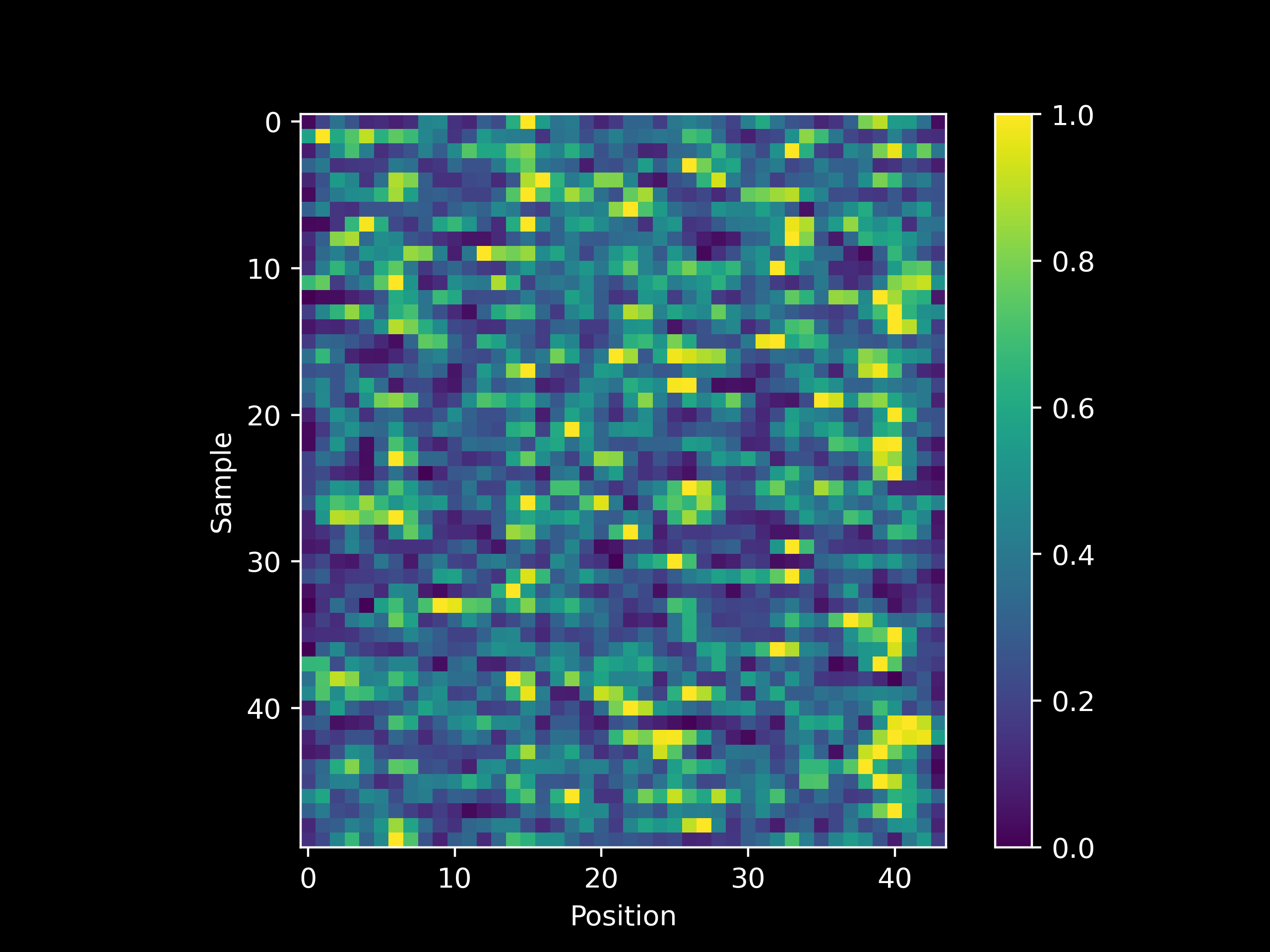
and see the source code for details on how to implement a heatmap-based visualization of model occlusion.

Using one of our controls, we may observe how a network ‘learns’ occlusion. Recalling that this dataset’s output is defined as

\[y = 10d\]

where $d$ is the Total Deliverers input, and observing that this input occupies the 24th through the 27th position (inclusive) in our input sequence (as there are fields of size 4, 1, 15, and 4 ahead of it and we are incrementing from 0 rather than 1), we expect the occlusiong attribution to be highest for these positions for the majority of inputs. Note that the Total Deliverers field is closely related to the Available Deliverers and Total Orders fields that follow it, as an increase in one is likely to affect the other two. In statistical terms, these fields are related via the underlying data generating distribution.

This means that although we may expect to see the Total Deliverers field as the most ‘important’ as measured using occlusion, a statistical model would be expected to also place fairly large attributions on the fields most similar to Total Deliverers. And if we observe occlusion values per character during a training run (200 epochs), indeed we see that this is the case (note how positions 24-27 are usually among the brightest in the following heatmap after training).

Attribution via Saliency

Occlusion is not the only way to obtain insight into which input elements are more or less important for a given output: another way we can learn this is to exploit the nature of the process of learning using a neural network or other similar deep learning models. This particular method is applicable to any model that uses a differentiable objective function, and thus is unsuitable for most tree-based machine learning models but is happily applicable to neural networks. Gradient-based input attribution is sometimes termed ‘saliency’.

The principle behind gradient based approaches to input attribution for neural network models is as follows: given some input, we can compute the model output and also the gradient of that output with respect to the weights and biases of the model. This gradient may then be back-propegated to the input layer of the network, as if the input were a parametric component of the neural network like the other layers. We then assess how the input contributes to the output’s gradient by multiplying the input gradient by the input itself.

\[g = \nabla_i f(x) * x\]

where $\hat{y} = f(x)$ is the model output, $x$ is the model input, $i$ is the input layer, and $g$ is the gradientxinput. Note that $\nabla_i f(x)$ and $x$ are both tensors, and as we want a tensor of the same size we use the Hadamard (element-wise) product, which when using torch.Tensor objects t1, t2, the Hadamard product may be obtained as t1 * t2.

The intuition behind this method is a little confusing for the researcher or engineer normally used to finding the gradient of an objective function with respect to a tunable parameter in a model, so before proceeding further let’s note the differences between this gradient used to interpret an input and the gradient used to train a model.

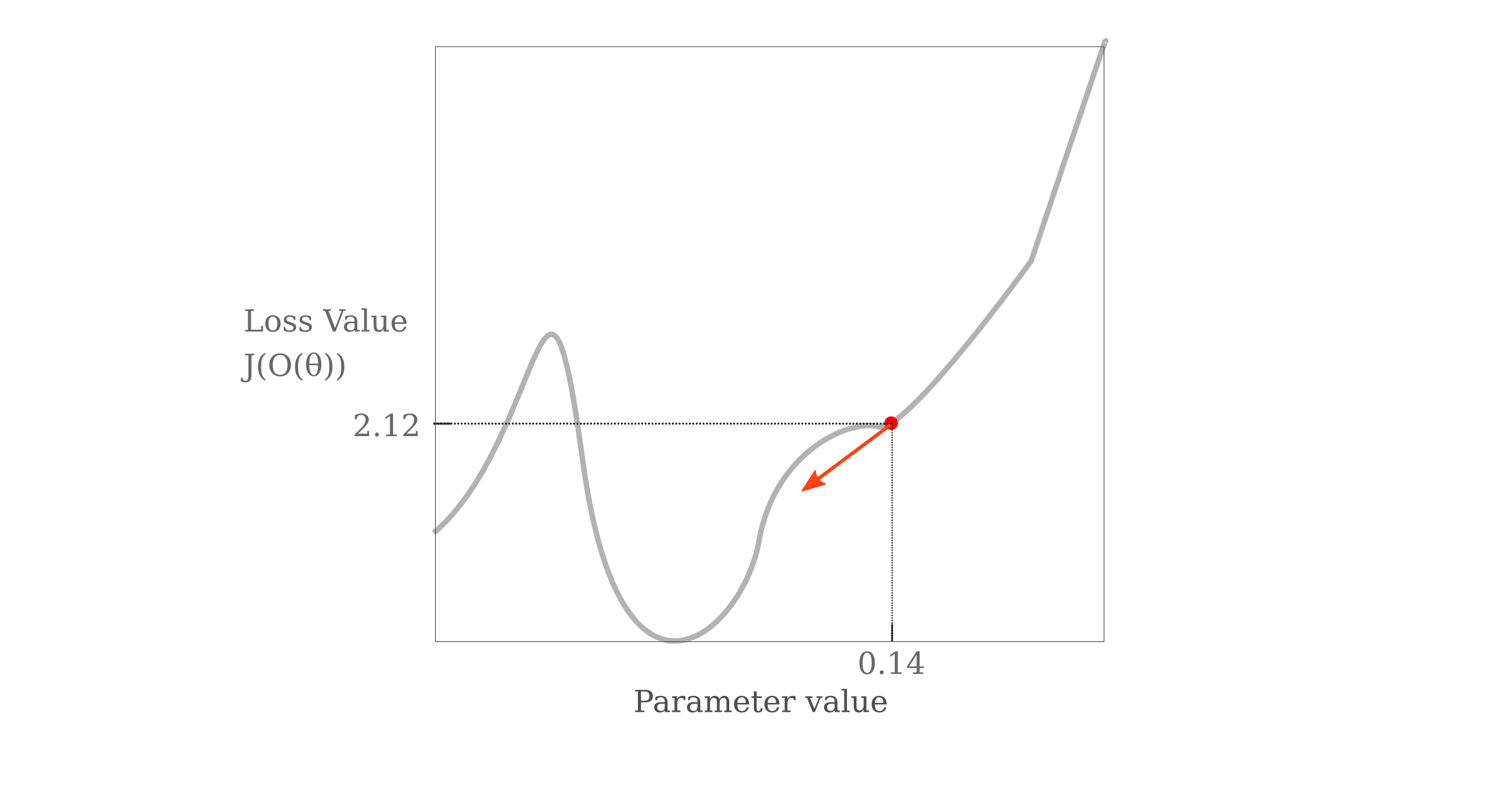
To summarize: the method by which the gradient of the objective (loss) function $J$ of the output given model a configuration $\theta$ denoted as $O(\theta)$ evaluated with respect to parameter $p$ is

\[g = \nabla_p J(O(\theta))\]

and we can imagine a landscape of this loss function with respect to one variable as a Cartesian graph. The opposite of the gradient tells us the direction (and partial magnitude) with which $p$ should be changed in order to minimize $J(O(\theta))$, which can be visualized as follows

For multiple variables, we can imagine this visualization as simply extending to multiple dimensions, with each parameter forming a basis in $\Bbb R^n$ space. The gradient’s component along the parameter’s axis forms the direction (with some magnitude information as well) in which that parameter should be changed.

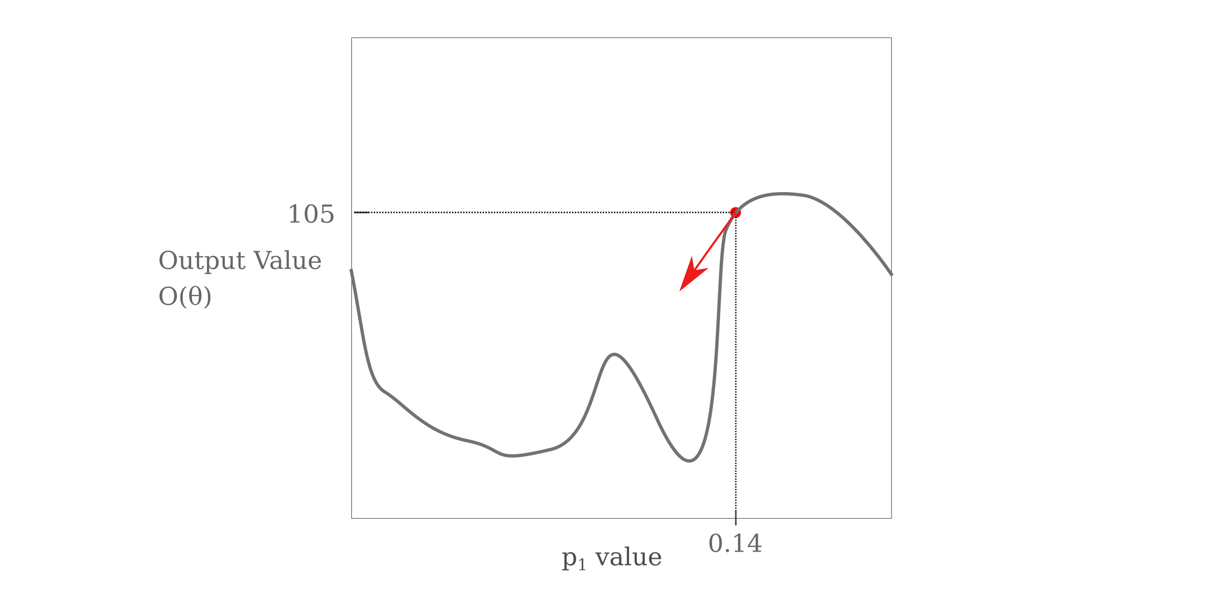
Now instead of evaluating the gradient with respect to the objective function, to determine how the output alone changes we can evaluate the gradient of the output $O(\theta)$ with respect to parameter $p$

\[g = \nabla_p O(\theta)\]

which can be visualized as

now to determine which parameter is more important for determining a given output, we can compare the gradients $g_1$ and $g_2$ which are computed with respect to $p_1$ and $p_2$, respectively

\[g_1 = \nabla_{p_1} O(\theta) \\ g_2 = \nabla_{p_2} O(\theta)\]

These can be visualized without resorting to multidimensional space as separate curves on a two dimensional plane (for any single value of $p_1$ and $p_2$ of interest) as follows:

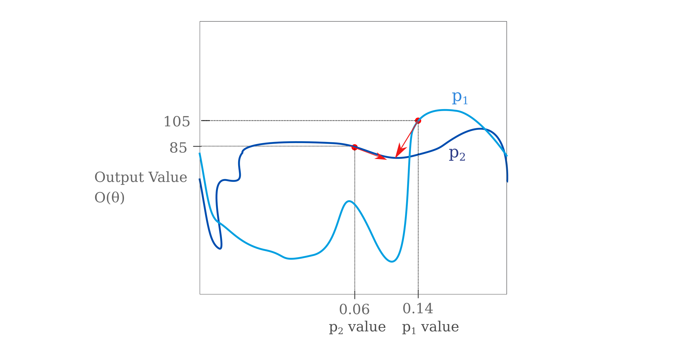
Where the red arrows denote $-g_1$ and $-g_2$ as gradients point in the direction of steepest ascent. In this particular example, $\vert g_1 \vert > \vert g_2 \vert$ as the slope of the tangent line is larger along the output curve for $p_1$ than along $p_2$ for the points of interest. In multidimensional space, we would be comparing the gradient vector’s components, where each parameter $p_n$ forms a basis vector of the space and the component is a projection of the gradient vector $g$ onto each basis.

The next step is to note that as we are most interested in finding how the output changes with respect to the input rather than with respect to the model’s true parameters, we treat the input itself as a parameter and back-propegate the gradient all the way to the input layer (which is not normally done as the input does not contain any parameters as normally defined). Thus in our examples, $(p_1, p_2) = (i_1, i_2)$ where $i_1$ is the first input and $i_2$ is the second.

Now that we have the gradient of the output with respect to the input, this gradient can be applied in some way to the input values themselves in order to determine the relation of the input gradient with the particular input of interest. The classic way to accomplish this is to use Hadamard multiplication, in which each vector element of the first multiplicand $v$ is multiplied by its corresponding component in the second multiplicand $s$

\[v = (v_1, v_2, v_3,...) \\ s = (s_1, s_2, s_3,...) \\ v * s= (v_1s_1, v_2s_2, v_3s_3, ...)\]

and all together, we have

\[g = \nabla_i f(x) * x\]

This final multiplication step is perhaps the least well-motivated portion of the whole procedure. When applied to image data in which each pixel (or in other words each input) can be expected to have a non-zero value, we would not expect to lose much information with Hadamard multiplication and furhtermore the process is fairly intuitive: brighter pixels (ie those with larger input values) that have the same gradient values as dimmer pixels are considered to be more important.

Thus we see that what occurs during the gradientxinput calculation is somewhat similar to that for the occlusion calculation, except instead of the input being perrured in some way, here we are using the gradient to find an expectation of how the output should change if one were to perturb the input in a particular way.

The following class method implements a slightly modified version of gradientxinput. Each 15 tensor inputs in sequence corresponds to one character, and so a natural way to accumulate the gradientxinput values is to first take the absolute values of the gradient components with respect to these inputs $\nabla_{ij}f(x)$, apply Hadamard multiplication to the corresponding input values $x_j$, and then sum up the resulting vector.

\[g = \sum_j \vert \nabla_{ij} f(x) \vert * x_j\]

A method implementing this version is as follows:

	def gradientxinput(self, input_tensor):
		"""
		 Compute a gradientxinput attribution score

		 Args:
		 	input: torch.Tensor() object of input
		 	model: Transformer() class object, trained neural network

		 Returns:
		 	gradientxinput: arr[float] of input attributions

		"""
		# enforce the input tensor to be assigned a gradient
		input_tensor.requires_grad = True
		output = self.model.forward(input_tensor)

		# only scalars may be assigned a gradient
		output_shape = 1
		output = output.reshape(1, output_shape).sum()

		# backpropegate output gradient to input
		output.backward(retain_graph=True)

		# compute gradient x input
		final = torch.abs(input_tensor.grad) * input_tensor
		saliency_arr = []
		s = 0
		for i in range(len(final)):
			if i % self.embedding_dim == 0 and i > 0: 
				saliency_arr.append(s)
				s = 0
			s += float(final[i])
		saliency_arr.append(s)

		# max norm
		maximum = 0
		for i in range(len(saliency_arr)):
			maximum = max(saliency_arr[i], maximum)

		# prevent a divide by zero error
		if maximum != 0:
			for i in range(len(saliency_arr)):
				saliency_arr[i] /= maximum

		return saliency_arr

which results in

Combining Occlusion and Gradientxinput

One criticism of pure gradient-based approaches such as gradientxinput is that they only apply to local information. This means that when we compute

\[\nabla_i f(x)\]

we only learn what happens when $i$ is changed by a very small amount $\epsilon$, which follows from the definition of a gradient. Techniques that attempt to overcome this locality challenge include integrated gradients and other such additive measures. But those methods have their own drawbacks (integrated gradients involve modifying the input such that the gradient-based saliency may exhibit dubious relevance to the original).

Happily, we already have a locality-free (non-gradient) based approach to attribution that we can add to gradientxinput in order to overcome this limitation. The intuition behind why occlusion is non-local is as follows: there is no a priori reason as to why a modification to the input at any position should yield an occluded input that is nearly indistinguishable from the original, and thus any results obtained from comparing the two images using our model do not apply only to the first image. Furthermore, the occlusion_size parameter provides a clear hyperparameter to prevent any incedental locality, as simply increasing this parameter size is clearly sufficient to increase the distance between $x_o$ and $x_c$ in the relevant latent space.

Thus it is not entirely inaccurate to think of gradientxinput as a continuous version of occlusion, as the former tells us what happens if we were to change the input by a very small amount whereas the latter tells us what would happen if we changed it by a large discrete amount.

We may combine occlusion with gradientxinput by simply averaging the values obtained at each position, and the result is as follows:

One may want to be able to have a more readable attribution than is obtained using the heatmaps above, This may be accomplished by averaging the attribution value of each character over a number of input examples, and then aggregating these values (using maximums or averages or another function) into single measurements for each field. An abbreviated implementation (lacking normalization and aggregation method choice) of this method is as follows:

	def readable_interpretation(self, count, n_observed=100, method='combined', normalized=True, aggregation='average'):
		"""
		...
		"""
		attributions_arr = []

		for i in range(n_observed):
			input_tensor = self.input_tensors[i]
			if method == 'combined':
				occlusion = self.occlusion(input_tensor)
				gradxinput = self.gradientxinput(input_tensor)
				attribution = [(i+j)/2 for i, j in zip(occlusion, gradxinput)]
			...
			attributions_arr.append(attribution)

		average_arr = []
		for i in range(len(attributions_arr[0])):
			average = sum([attribute[i] for attribute in attributions_arr])
			average_arr.append(average)
		...
		if aggregation == 'average':
			final_arr = []
			index = 0
			for i, field in zip(self.taken_ls, self.fields_ls):
				sum_val = 0
				for k in range(index, index+i):
					sum_val += average_arr[k]
				final_arr.append([field, sum_val/k])
				index += i
		...
		plt.barh(self.fields_ls, final_arr, color=colors, edgecolor='black')
		...
		return

(note that the working version may be found in the source code)

For the trained network shown above, this yields

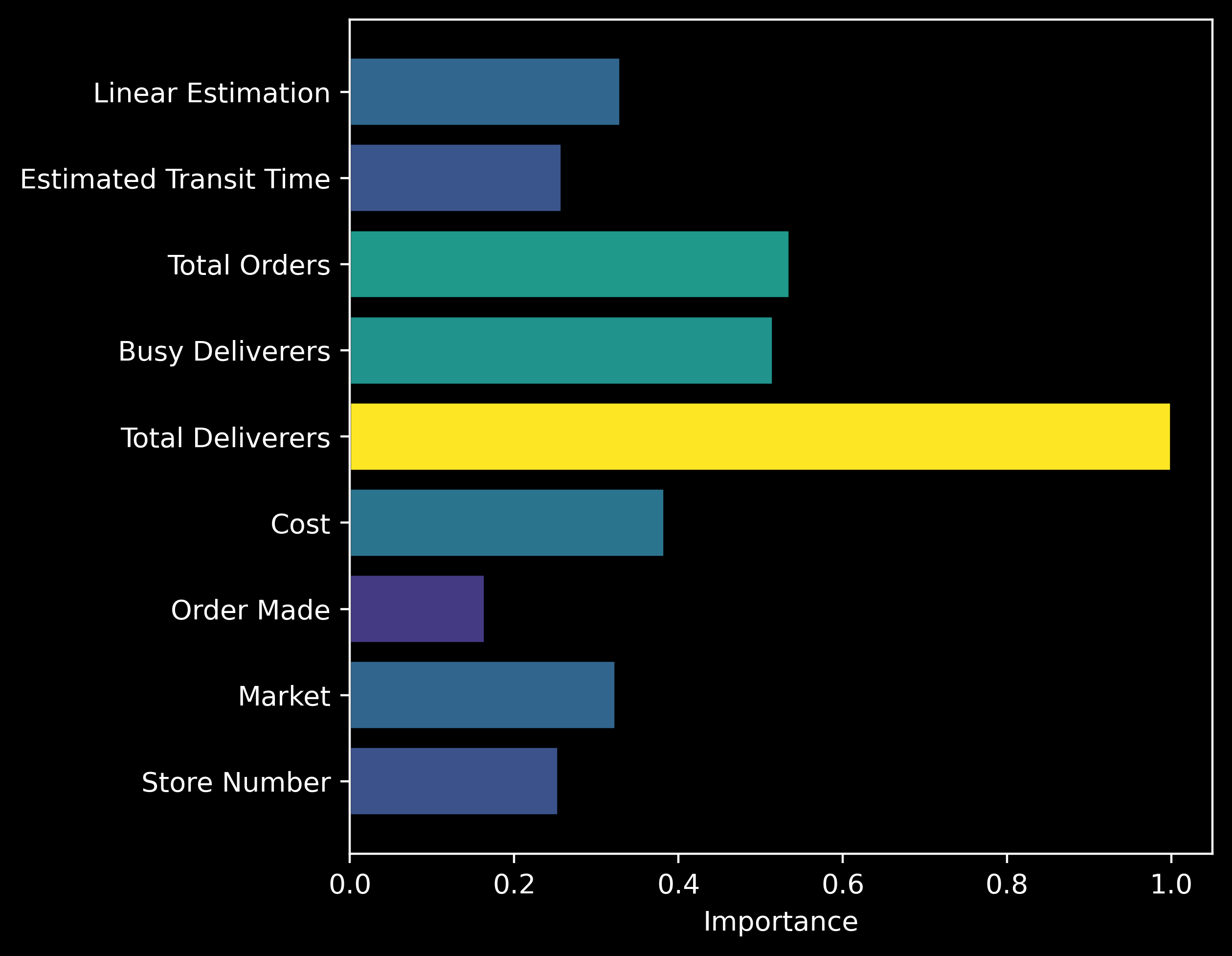
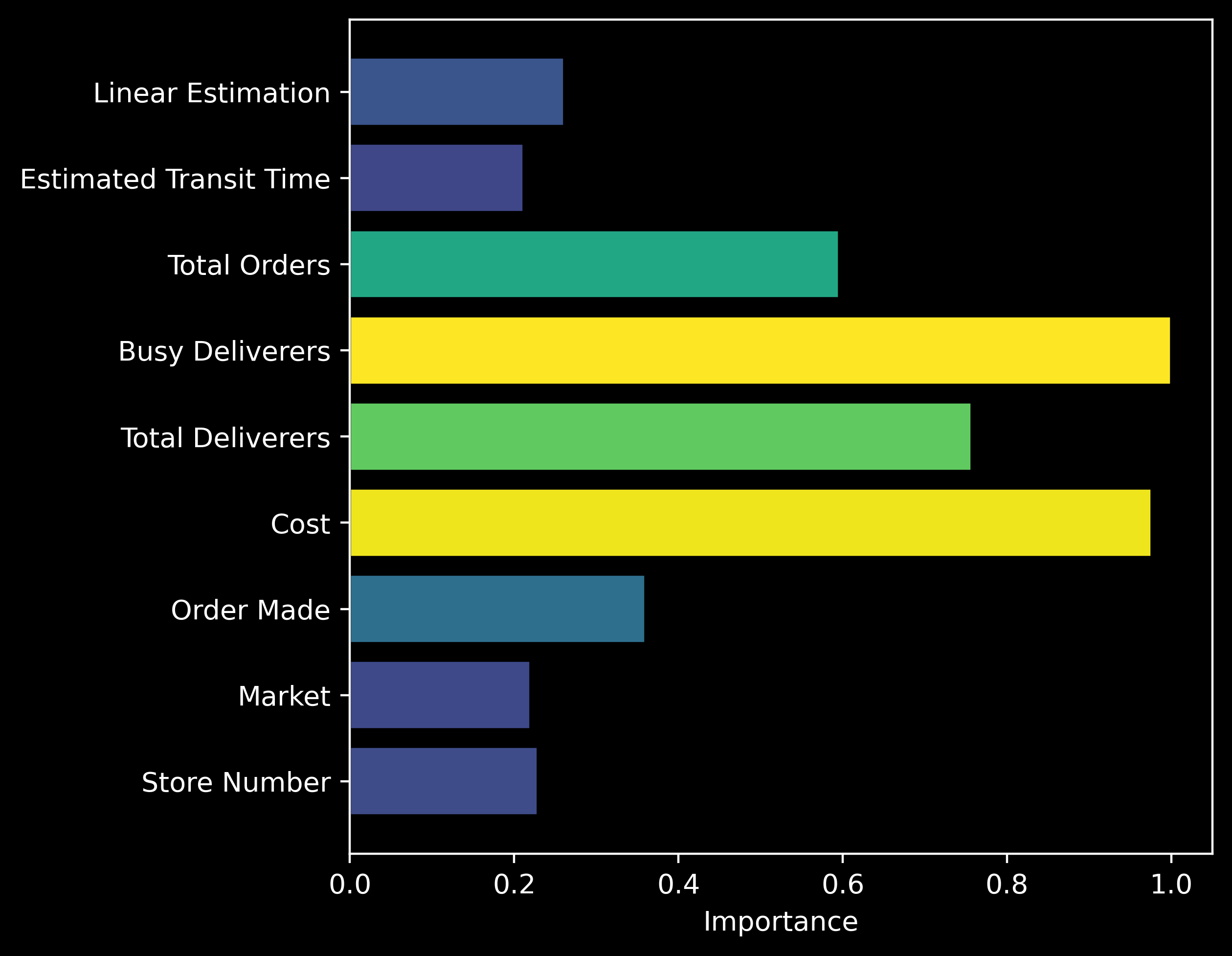
and the correct input is attributed to be the most important, so our positive control indicates success. What about a slightly more realistic function in which multiple input fields contribute to the output? Recall that in our nonlinear control function, the output $y$ is determined by the function

\[y = (c/100) * b\]

where $b$ is the Busy Deliverers input and $c$ is the Cost input. During training we can see that the expected (20-23 and 28-31 inclusive) positions are the ones that obtain the highest attribution values for most inputs:

and when the average attribution per input is calculated, we see that indeed the correct fields contain the highest attribution.

Now we can apply this method to our original problem of finding which input are important for predicting a delivery time.