Structured Sequence Inputs

This page is part I of II, for part II see here.

Relying on the ability of deep learning to form representations of an input, we explore neural networks’ ability to learn from structured abstract sequential inputs.

Introduction and background

Deep learning here is defined as a type of machine learning in which the input is represented in successive layers, with each layer being a distributed representation of the previous. This allows for the approximation of very complicated functions by

Deep learning approaches are often touted for having greater accuracy than other machine learning approaches, and for certain problems this is indeed true. Tasks such as visual object recognition, speech transcription or language translation are among those problems at which deep learning approaches are currently the most effective at among all machine learning techniques, and for some problems the efficacy of deep learning is far beyond what has been achieved by other methods.

The kinds of tasks mentioned in the last paragraph are sometimes called ‘AI-complete’, which is an analogy to the ‘NP-complete’ problems that are as hard as all other NP-complete problems with regards to computational complexity reduction. These tasks are quite difficult for traditional machine learning, but are often approachable using deep learning methods, and indeed most research on the topic since the seminal papers of 2006 have been focused on the ability of deep learning to out-perform other methods on previously-unseen data.

This page focuses on a different but related benefit of deep learning: the ability to learn an arbitrary representation of the input, allowing one to use one model for a very wide array of possible problems. The interpretability, or the ability to understand how the model arrives at any prediction, of this flexible approach is then explored.

Abstract sequence modeling

Deep learning approaches such as neural networks are able to learn a wide array of functions (although there are certainly limits to what any machine learning approach is able to approximate, see here for more details

Work on this topic was in part inspired by the finding that the large language model GPT-3 was able to learn arithmetic. The research question: given that a large language model is able to learn simple functions on sequential character inputs, can a smaller model learn simple and complex functions using language-like inputs as well?

The importance of this question is that if some model were to be able to learn how to approximate certain functions on an input comprising something as general as a sequence of characters, a machine learning practitioner would be able to avoid the often difficult process of formatting each feature for each dataset of interest. In the following sections, we shall see that the answer to this question is yes.

Input Flexibility

To start with, we will use a small dataset and tailor our approach to that specific dataset before then developing a generalized approach that is capable of modeling any abitrary grid of values. Say we were given the following training data in the form of a design matrix:

Market	Order Made	Store Number	Cost	Total Deliverers	Busy Deliverers	Total Orders	Estimated Transit Time	Linear Estimation	Elapsed Time
1	2015-02-06 22:24:17	1845	3441	33	14	21	861	3218	3779
2	2015-02-10 21:49:25	5477	1900	1	2	2	690	2818	4024
3	2015-01-22 20:39:28	5477	1900	1	0	0	690	3090	1781
3	2015-02-03 21:21:45	5477	6900	1	1	2	289	2623	3075

We have a number of different inputs and the task is to predict Elapsed Time necessary for a delivery. The inputs are mostly integers except for the Order Made feature, which is a timestamp. The names of the third-to-last and second-to-last columns indicate that we are likely developing a boosted model, or in other words a model that takes as its input the outputs of another model.

For some perspective, how would we go about predicting the Elapsed Time value if we were to apply more traditional machine learning methods? As most features are numerical and we want an integer output, the classical approach would be to hand-format each feature, apply normalizations as necessary, feed these into a model, and recieve an output that is then used to train the model. This was how the Linear Estimation column was made: a multiple ordinary least squares regression algorithm was applied to a selection of formatted and normalized features with the desired output. More precisely, we have fitted weight $w \in \Bbb R^n$ and bias (aka intercept) $b \in \Bbb R^n$ vectors such that the predicted value $\hat {y}$ is

\[\hat {y} = w^Tx + b \tag{1}\]

where $x$ is a (6-dimensional) vector containing the formatted inputs of the relevant features we want to use for predicting Elapsed Time, denoted $y$. The parameters of $w, b$ for linear models usually by minimizing the mean squared error

\[MSE = \frac{1}{m} \sum_i (\hat {y_i} - y_i)^2\]

Other more sophisticated methods may be employed in a similar manner in order to generate a scalar $\hat y$ from $x$ via tuned values of parameter vectors $w$ and $b$. Now consider what is necessary for our linear model to perform well: first, that the true data generating distribution is approximately linear, but most importantly for this page that the input vector $x$ is properly formatted to avoid missing values, differences in numerical scale, differences in distribution etc.

When one seeks to format an input vector, there are usually many decision that one has to make. For example: what should we do with missing values: assign a placeholder, or simply remove the example from our training data? What should we do if the scale of one feature is orders of magnitude different than another? Should we enforce normality if the distribution for each feature, and if so what mean and standard deviation should we apply? How should we deal with categorical inputs, as only numerical vectors are accepted in the linear model? For categorical inputs with many possible options, should we perform dimensionality reduction to attempt to capture most of the information present in a lower-dimensional form? If so, what is the minimum number of options we should use and what method should we employ: a neural network-based embedding, sparse matrix encoding, or something else?

These questions and more are all implicitly or explicitly addressed when one formats data for a model such as this: the resulting vector $x$ is composed of ‘hand-designed’ features. But how do we know that we have made the optimal decisions for formatting each input? If we have many options of how to format many features, it is in practice impossible to try each combination of possible formats and therefore we do not actually know which recipe will be optimal.

The approach of deep learning is to avoid hand-designed features and instead allow the model to learn the optimal method of representing the input as part of the training process. A somewhat extreme example of this would be to simply pass a transformation (encoding) $f$ of the raw character input as our feature vector $x$. For the first example in our training data above, this equates to some function of the string as follows:

\[x = f(1 \;2015-02-06 \; 22:24:17 \;1845 \;3441 \;33 \;14 \;21 \;861 \;3218)\]

There are a number of different functions $f$ may be used to transform our raw input into a form suitable for a deep learning program. In the spirit of avoiding as much formatting as possible, we can assign $f$ to be a one-hot character encoding, and then flatten the resulting tensor if our model requires it. One-hot encodings take an input and transform this into a tensor of size $\vert n \vert$ where $n$ is the number of possible categories, where the position of the input among all options determines which element of the tensor is $1$ (the rest are zero). For example, a one-hot encoding on the set of one-digit integers could be

\[f(0) = [1, 0, 0, 0, 0, 0, 0, 0, 0, 0] \\ f(1) = [0, 1, 0, 0, 0, 0, 0, 0, 0, 0] \\ f(2) = [0, 0, 1, 0, 0, 0, 0, 0, 0, 0] \\ \vdots \\ f(9) = [0, 0, 0, 0, 0, 0, 0, 0, 0, 1]\]

Note that it does not matter which specific encoding method we use, and that any order of assignment will suffice (for example, we could swap $f(0)$ and $f(1)$). Nor does it particularly matter that we place a $1$ in the appropriate position for our tensor: any constant $c$ would work, as long as this constant is not changed between inputs. What is important is that each category of input is linearly independent of all other categories, meaning tat we cannot apply some compression such as

\[f(0) = [1, 0] \\ f(1) = [0, 1] \\ f(2) = [1, 1] \\ \vdots\]

or even simply assign each value to a single tensor,

\[f(0) = [0] \\ f(1) = [1] \\ f(2) = [2] \\ \vdots\]

These and any other methods of encoding such that each input category is no longer linearly independent of each other (and not normed to one constant $c$) are generally bad because it introduces information about the input $x$ that is not likely to be true: if we were encoding alphabetical characters instead of integers, each character should be ‘as different’ from each other character but this would not be the case if we applied a linearly dependent encoding.

For some perspective, we can compare this input method to a more traditional approach that is currently used for deep learning. The strategy for that approach is as follows: inputs that are low-dimension may be supplied as one-hot encodings (or as basis vectors of another linearly independent vector space) and inputs that are high-dimensional (such as words in the english language) are first embedded using a neural network, and the result is then given as an input for the chosen deep learning implementation.

Embedding is the process of attempting to recapitulate the input on the output, while using less information that originally given. The resulting embedding, also called a latent space, is no longer generally linearly independent but instead contains information about the input itself: for example, vectors for the words ‘dog’ and ‘cat’ would be expected to be more similar to each other than the vectors ‘dog’ and ‘tree’.

Such embeddings would certainly be possible for our character-based approach, and may even be optimal, but the following intuition may explain why they are not necessary for successful application of our sequential encoding: we know that any deep learning model will reduce dimensionality to 0 (in the case of regression) or $n$ (for $n$ categories) depending on the output, so we can expect the model itself to perform the same tasks that an embedding would. This is perhaps less efficient than separating out the embedding before then training a model on a given task, but it turns out that this method can be employed quite successfully.

To summarize, we can bypass not only the need for hand-chosen formatting and normalization procedures but also for specific embeddings when using a sequential character-based input approach.

Weaknesses of recurrent neural net architectures

One choice remains: how to deal with missing features. For models such as (1), this may be accomplished by simply removing training examples that exhibit missing features, and enforcing the validation or test datasets to have some value for all features. The same approach could be applied here, but such a strategy could lead to biased results. What happens when not only a few but the majority of examples both for training and testing are missing data on a certain feature? Removing all examples would eliminate the majority of information in our training dataset, and is clearly not the best way to proceed.

Perhaps the simplest way to proceed would be to assign our sequence-to-tensor mapping function $f$ to map an empty feature to an empty tensor. For example, suppose we wanted to encode an $x_i$ which was missing the first feature value of $x_c$:

\[x_c = f(1 \; 2015-02-06 \; 22:24:17 \;1845 \;3441 \;33 \;14 \;21 \;861 \;3218) \\ x_i = f( \; 2015-02-06 \; 22:24:17 \;1845 \;3441 \;33 \;14 \;21 \;861 \;3218)\]

in this case $x_c = x_i$ except for the first 10 elements of $x_c$, which $x_i$ omits. The non-concatenated tensors would be

\[x_c = [[0,1,0,0,0,0,0,0,0,0],[0,0,1,...] ...]\\ x_i = [[],[0,0,1,...] ...]\]

which means that the concatenated versions begin as $[0,1,0…]$ for $x_c$ and $[0,0,1,…]$ for $x_i$, resulting in a variable-length $x$.

A specific class of deep learning models have been designed for variable-length inputs. These are recurrent neural networks, and they operate by examining each input sequentially (ie for $x_c$ the network would first take an input as $[0,1,0,0,0,0,0,0,0,0]$), using that input to update the activations for each neuron according the the weights $w$ and biases $b$ present in that network, and then perhaps generating an output which can be viewed as an observation of the activations of the final layer of neurons.

For our regression problem, the only output that we would need to be concerned with is the output after the last input was recieved by the network. This output would then be used for loss back-propegation according to the gradient of the loss.

One difficulty with recurrent neural networks is that they may suffer from exploding gradients: if each input adds to the previous, so can the gradient from each output leading to exceptionally large gradients for long sequences and thus difficulties during stochastic gradient descent. This particular problem may be remedied a number of different ways, one of which involves gating the activations for each sequential input. Another problem is that because network activations are added together, pure recurrent networks often have difficulty ‘remembering’ information fed into the network at the start of the sequence whilst nearing the end.

Both of the problems in the last paragraph are addressed using the Long Short-term Memory recurrent architecture, which keeps both short-term as well as a long-term memory modules in the form of neurons that are activated and gated. However, even these and other modified recurrent nets do not address perhaps the most difficult problem of recurrence during training: the process has a tendancy to ‘forget’ older examples relative to non-recurrent architectures, as there is $n^2$ distance between the last update and first update with respect to parameter activations. See this page for more informatino on this topic.

That said, recurrent neural net architectures can be very effective deep learning procedures. But there is a significant drawback to using them for our case: we lose information on the identity of each feature. To explain why this is, imagine observing the following tensor as the first input: $[0,1,0…]$. There is not way a priori for you to know which feature this input tensor corresponds to, whereas in our grid of values above, we certainly would know which column (and therefore which feature) an empty value was located inside.

The importance of maintaining positional information for tasks such as these has been borne out by experiment: identical LSTM-based neural networks perform far better with respect to minimization of test error using input functions $f$ that retains positional information compared to $f$ that do not.

Structured sequence input encoding

How do we go about preserving positional information for a sequence in order to maintain feature identity for each input element? A relatively simple but effective way of doing this is to fix the number of elements that are assigned to be a constant value $c$, and then to provide a place-holder value $v$ for however many elements that a feature is missing. In our example above, this could be accomplished by adding an eleventh element to each tensor (which we can think of as denoting ‘empty’) and performing one-hot encoding using this expanded vocabulary,

\[x_c = [[0,1,0,0,0,0,0,0,0,0,0],[0,0,1,...] ...]\\ x_i = [[0,0,0,0,0,0,0,0,0,0,1],[0,0,1,...] ...]\]

The important thing here is to keep the element denoting ‘empty’ to be one that is rarely if ever used to denote anything else. For example, if we were to use the tensor for $f(0)$ to denote an empty character, we would lose information if $0$ were found in any of the features because a priori the model cannot tell if the tensor $f(0)$ denotes a zero element or an empty element.

This structured input can be implemented as follows: first we import relevant libraries and then the class Format is specified. Note that source code for this page may be found here.

# fcnet.py
# import standard libraries
import string
import time
import math
import random

# import third-party libraries
import numpy as np 
import matplotlib.pyplot as plt 
import pandas as pd
from sklearn.utils import shuffle

import torch
import torch.nn as nn

class Format:

	def __init__(self, file, training=True):

		df = pd.read_csv(file)	
		df = df.applymap(lambda x: '' if str(x).lower() == 'nan' else x)
		df = df[:10000]
		length = len(df['Elapsed Time'])
		self.input_fields = ['Store Number', 
				'Market', 
				'Order Made',
				'Cost',
				'Total Deliverers', 
				'Busy Deliverers', 
				'Total Orders',
				'Estimated Transit Time',
				'Linear Estimation']

		if training:
			df = shuffle(df)
			df.reset_index(inplace=True)

			# 80/20 training/validation split
			split_i = int(length * 0.8)

			training = df[:][:split_i]
			self.training_inputs = training[self.input_fields]
			self.training_outputs = [i for i in training['positive_two'][:]]

			validation_size = length - split_i
			validation = df[:][split_i:split_i + validation_size]
			self.validation_inputs = validation[self.input_fields]
			self.validation_outputs = [i for i in validation['positive_two'][:]]
			self.validation_inputs = self.validation_inputs.reset_index()

		else:
			self.training_inputs = self.df # not actually training, but matches name for stringify

Then in this class we implement a method that converts each row of our design matrix into a sequence of characters, which will be used as an argument to $f()$.

class Format:
  ...
  
  def stringify_input(self, index, training=True):
		"""
		Compose array of string versions of relevant information in self.df 
		Maintains a consistant structure to inputs regardless of missing values.

		Args:
			index: int, position of input

		Returns:
			array: string: str of values in the row of interest

		"""


		taken_ls = [4, 1, 8, 5, 3, 3, 3, 4, 4]

		string_arr = []
		if training:
			inputs = self.training_inputs.iloc[index]
		else:
			inputs = self.validation_inputs.iloc[index]

		fields_ls = self.input_fields
		for i, field in enumerate(fields_ls):
			entry = str(inputs[field])[:taken_ls[i]]
			while len(entry) < taken_ls[i]:
				entry += '_'
			string_arr.append(entry)

		string = ''.join(string_arr)
		return string

Now we implement another class method which will perform the task of $f()$, ie of converting a sequence of characters to a tensor. In this particular example, we proceed with concatenating each character’s tensor into one in the tensor = tensor.flatten() line because we are going to be feeding our inputs into a simple fully-connected feed-forward neural network architecture.

	@classmethod
	def string_to_tensor(self, input_string):
		"""
		Convert a string into a tensor

		Args:
			string: str, input as a string

		Returns:
			tensor: torch.Tensor() object
		"""
		
		places_dict = {s:i for i, s in enumerate('0123456789. -:_')}
		
		# vocab_size x batch_size x embedding dimension (ie input length)
		tensor_shape = (len(input_string), 1, 15) 
		tensor = torch.zeros(tensor_shape)

		for i, letter in enumerate(input_string):
			tensor[i][0][places_dict[letter]] = 1.

		tensor = tensor.flatten()
		return tensor 

and now we can assemble a neural network. Here we implement a relatively simple fully-connected network by inheriting from the torch.nn.Module library and specify a 5-layer (3 hidden layer) architecture.

 class MultiLayerPerceptron(nn.Module):

	def __init__(self, input_size, output_size):

		super().__init__()
		self.input_size = input_size
		hidden1_size = 500
		hidden2_size = 100
		hidden3_size = 20
		self.input2hidden = nn.Linear(input_size, hidden1_size)
		self.hidden2hidden = nn.Linear(hidden1_size, hidden2_size)
		self.hidden2hidden2 = nn.Linear(hidden2_size, hidden3_size)
		self.hidden2output = nn.Linear(hidden3_size, output_size)
		self.relu = nn.ReLU()
		self.dropout = nn.Dropout(0.3)

	def forward(self, input):
		"""
		Forward pass through network

		Args:
			input: torch.Tensor object of network input, size [n_letters * length]

		Return: 
			output: torch.Tensor object of size output_size

		"""

		out = self.input2hidden(input)
		out = self.relu(out)
		out = self.dropout(out)

		out = self.hidden2hidden(out)
		out = self.relu(out)
		out = self.dropout(out)

		out = self.hidden2hidden2(out)
		out = self.relu(out)
		out = self.dropout(out)

		output = self.hidden2output(out)
		return output

Note that for the positive control experiments below, dropout is disabled during training.

This architecture may be understood as accomplishing the following: the last layer is equivalent to a linear model $y=w^Tx’ + b$ on the final hidden layer $x’$ as an input, meaning that the hidden layers are tasked with transforming the input vector $x$ into a representation $x’$ that is capable of being modeled by (1).

Finally we can choose an objective (loss) function and an optimization procedure. Here we use L1 loss rather than MSE loss as our objective function because it usually results in less overfitting (as it fits a $\hat y$ to the median rather than the mean of an appropriate input $x$)

\[L^1_{loss} = \frac{1}{m} \sum_i \vert \hat {y_i} - y_i \vert\]

where $m$ is the number of elements indexed by $i$. Here we use Adaptive moment estimation, a variant of stochastic gradient descent, as our optimization procedure. Also employed is gradient clipping, which prevents gradient tensors with poor condition number from adversely affecting optimization.

	def __init__(self,...):
	self.optimizer = torch.optim.Adam(self.model.parameters(), lr=1e-4)
	...
	
	def train_minibatch(self, input_tensor, output_tensor, minibatch_size):
		"""
		Train a single minibatch

		Args:
			input_tensor: torch.Tensor object 
			output_tensor: torch.Tensor object
			optimizer: torch.optim object
			minibatch_size: int, number of examples per minibatch
			model: torch.nn

		Returns:
			output: torch.Tensor of model predictions
			loss.item(): float of loss for that minibatch

		"""

		output = self.model(input_tensor)
		output_tensor = output_tensor.reshape(minibatch_size, 1)
		loss_function = torch.nn.L1Loss()
		loss = loss_function(output, output_tensor)

		self.optimizer.zero_grad() # prevents gradients from adding between minibatches
		loss.backward()

		nn.utils.clip_grad_norm_(self.model.parameters(), 0.3)
		self.optimizer.step()

		return output, loss.item()

Controls

Before applying our model to the dataset in question, we can directly assess the efficacy or our sequential character encoding method by applying the model to what in experimental science is known as a positive control. This is a (usually synthetic) dataset in which the desired outcome is known beforehand, such that if the experimental apparatus were successful in being able to perform its function then we would be able to arrive at some specific output.

In this case, we are interested in determining whether or not this relatively small neural network is capable of learning defined functions, in contrast to the as-yet undefined function that determines the actual delivery time (together with any Bayesian error). Our first control is as follows:

Market	Order Made	Store Number	Cost	Total Deliverers	Busy Deliverers	Total Orders	Estimated Transit Time	Linear Estimation	Control Output
1	2015-02-06 22:24:17	1845	3441	33	14	21	861	3218	330
2	2015-02-10 21:49:25	5477	1900	1	2	2	690	2818	10
3	2015-01-22 20:39:28	5477	1900	1	0	0	690	3090	10
3	2015-02-03 21:21:45	5477	6900	1	1	2	289	2623	10

where the function is

\[y = 10d\]

where $d$ is the Total Deliverers input. We can track test (previously unseen) accuracy during training on any regression by plotting the actual value (x-axis) agains the model’s prediction (y-axis): a perfect model will have all points aligned on the line $y=x$. Plotting the results of the above model on a test (unseen during training) dataset every 23 epochs, we have

so clearly for this control function, the model arrives at near-perfect accuracy fairly quickly. It is important here to note that this is a much more difficult problem for the model than at first it may seem because of the encoding method: rather than simply assign an appropriate weight to an input neuron encoding $d$ instead the model must learn to decode the encoding function, and then apply the appropriate weight to the decoded value. In effect, we are enforcing a distributed representation of the input because the encoding method itself is distributed (here $4*15=60$ tensor values rather than $1$).

We can also experiment with the network learning a more complicated rule, this time the non-linear (with respect to the input) mapping

\[y = (c/100) * b\]

where $b$ is the Busy Deliverers input and $c$ is the Cost input field. Once again, the model is capable of very accurate estimations on the test dataset (actual outputs on the x-axis and expected outputs on the y-axis)

with the trained model achieving $R^2>0.997$, meaning that less than $0.3%$ of the variation in the actual value was not accounted for by the model’s prediction. Further observation shows that a small number of points are poorly predicted by the model, to be specific the trained model yields far lower expected values compared to the actual $y$ value. Why could this be? On explanation is that this nonlinear function is more difficult to fit for our model, but this does not seem likely given that the model was capable of fitting a quite complicated nonlinear function to the first control. This is because the input encoding requires the model to be able to decode a sequence of characters into a number, such that the model must learn a far more complicated function than $y=10d$.

If the model is capable Observing the Cost input, we find that a small number of examples contain 5 digit cost values. Our encoding scheme only takes 4 characters from that input, which results in ambiguous information being fed to the model, as $13400$ and $1340$ would be indistinguishable. We can rectify this by assigning the Cost input to take 5 characters as follows:

taken_ls = [4, 1, 8, 5, 3, 3, 3, 4, 4]

which yields

and indeed accuracy has been greatly increased for these examples. There is some experimental evidence that the estimation accuracy for both positive controls diminishes as the number of training examples increases, or in symbols $\sum_i \hat {y_i} - y_i \to 0$ as $i \to \infty$.

These examples show that certain known functions on the input are capable of being approximated quite well by a structured sequence -based encoding method when fed to a relatively small fully connected feedforward neural network.

Generalization and language model application

The greatest advantage of the structured sequence input is its flexibility: because all inputs are converted to a single data type automatically, the experimentor does not need to determine the method by which each input is encoded. Thus we are able to combine heterogeneous inputs not only consisting of integers and timestamps but also categorical variables, language strings, images, and even audio input (provided that it has been digitized).

Up to now, the input method has been designed with only one problem in mind. The number of elements per input field was specified as

taken_ls = [4, 1, 15, 5, 4, 4, 4, 4, 4]

which is only applicable to that particular dataset. This may be generalized a number of different ways, but one is as follows: we take either all or else a portion (short=True) of each input field, the number of elements of which is denoted by n_taken (which must be larger than the longest element if all characters in an input field are to be used)

	def stringify_input(self, input_type='training', short=True, n_taken=5, remove_spaces=True):
		"""
		Compose array of string versions of relevant information in self.df 
		Maintains a consistant structure to inputs regardless of missing values.

		kwargs:
			input_type: str, type of data input requested ('training' or 'test' or 'validation')
			short: bool, if True then at most n_taken letters per feature is encoded
			n_taken: int, number of letters taken per feature
			remove_spaces: bool, if True then input feature spaces are removed before encoding

		Returns:
			array: string: str of values in the row of interest

		"""
		n = n_taken

		if input_type == 'training':
			inputs = self.training_inputs

		elif input_type == 'validation':
			inputs = self.val_inputs

		else:
			inputs = self.test_inputs

		if short == True:
			inputs = inputs.applymap(lambda x: '_'*n_taken if str(x) in ['', '(null)'] else str(x)[:n])
		else:
			inputs = inputs.applymap(lambda x:'_'*n_taken if str(x) in ['', '(null)'] else str(x))

		inputs = inputs.applymap(lambda x: '_'*(n_taken - len(x)) + x)
		string_arr = inputs.apply(lambda x: '_'.join(x.astype(str)), axis=1)

		return string_arr

We assemble the strings into tensors in a similar manner as above for the string_to_tensor method, except that the dataset’s encoding may be chosen to be any general set. For example, if we were except encoding to all ascii characters rather than only a subset. This makes the dimension of the model’s encoding rise from 15 to 128 using places_dict = {s:i for i, s in enumerate([chr(i) for i in range(128)])}.

A boolean argument Flatten may also be supplied, as some deep learning models are designed for language-like inputs

	@classmethod
	def string_to_tensor(self, string, flatten):
		...
		if flatten:
			tensor = torch.flatten(tensor)
		return tensor

Structured sequence inputs are in some way similar to natural languages: both contain a string of characters, of which only a small subset of all possible sequences ever appears as an example. One may therefore ask the question: can we apply specialized deep learning architectures developed for natural language processing to our structured sequence modeling tasks?

One architecture that is currently in use for large-scale language modeling is the transformer, which is a feedforward style network developed from recurrent neural network architectures that incorperated a concept called ‘self-attention’. In a self-attention module, each input (usually a word but here will be a letter) is associated with three vectors $K, Q, V$ for Key, Query, and Value that are produced from learned weight matricies $W^K, W^Q, W^V$. Similarity between inputs to the first element (denoted by the vector $\pmb{s_1}$) is calculated by finding the dot product (denoted $*$) of one element’s query vector with all other element’s key vectors

\[\pmb{s_1} = (q_1*k_1, q_1*k_2, q_1*k_3,...)\]

before a linear function is applied to each element followed by a softmax transformation to the vector $\pmb{s_1}$ to make $\pmb{s_1’}$. Finally each of the resulting scalar components of $s$ are multiplied by the corresponding value vectors for each input $V_1, V_2, V_3,…$ and the resulting vectors are summed up to make the activation vector $\pmb{z_1}$ that is the same dimension as $V_1$

\[\pmb{s_1'} = \mathbf{softmax} \; ((q_1*k_1)/ \sqrt d, (q_1*k_2)/ \sqrt d, (q_1*k_3)/ \sqrt d,...) \\ \pmb{s_1'} = (s_{11}', s_{12}', s_{13}',...) \\ \pmb{z_1} = V_1 s_{11}' + V_2 s_{12}' + V_3 s_{13}'+ \cdots\]

The transformer is based on multi-head attention, which means that multiple self-attention $z_1$ vectors are obtained (and thus multiple $W^K, W^Q, W^V$ vectors are learned) for each input. The multi-head attention is usually followed by a layer normalization and fully connected layer (followed by another layer normalization) to make one transformer encoder. Multiple encoder modules are usually stacked sequentially, and for this page we will be using the following architecture that employs 3 encoder modules that feed into a single fully connected layer.

The transformer encoder and decoder modules are reportedly not particularly effective at retaining positional information from the input. This is presumably due to the addition step used to make $\pmb{z_1}$, as after this step the resulting vector contains information of which other element is most similar to $s_1$, but not where that element was found. To remedy this, a positional encoding is usually applied to the input prior to feeding the input to the transformer encoder. The positional encoding may be performed a number of different ways, but one that is most common is to simply add the values of periodic functions such as $\sin, \cos$ to the input directly. See the code repo for an implementation of this kind of positional encoding.

An aside: it has been claimed that positional encoding is necessary for transformer-style architectures because they lose practically all positional information during the multi-head attention stage. This is not strictly true, as can be shown experimentally: simply permuting any given input usually yields a different output from the transformer encoder, meaning that order does indeed determine the output. Indeed, simply removing positional encoding does not result in significant reductions in test accuracy, suggesting that for this application positional encoding is superfluous.

All together, the architecture is as follows:

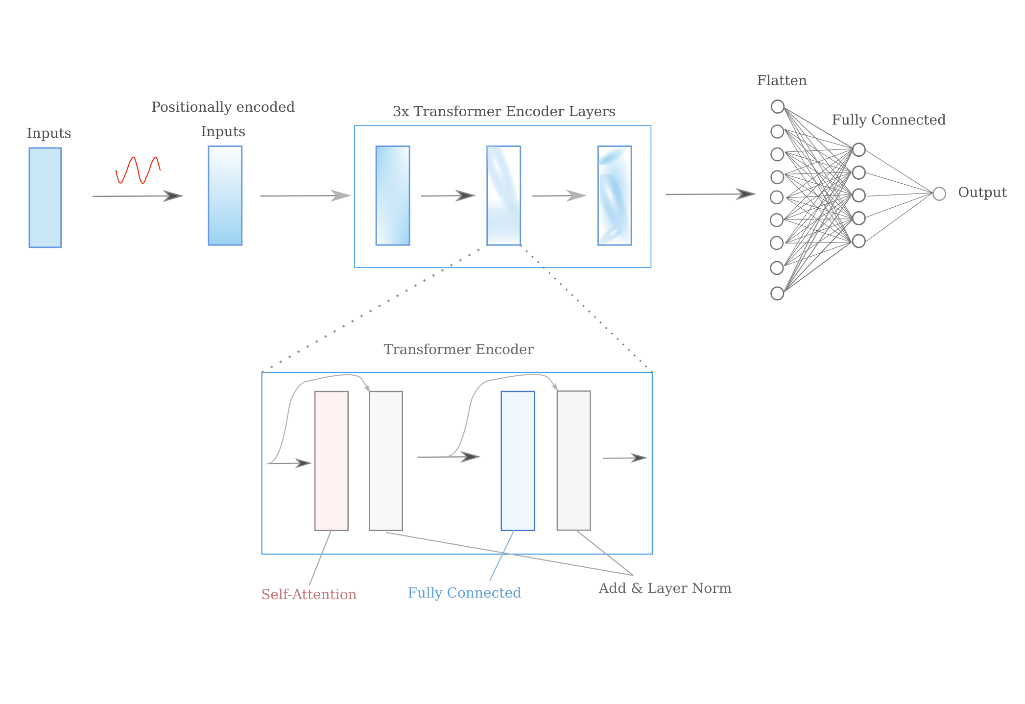
and the implementation for this architecture is as follows:

class Transformer(nn.Module):
	"""
	Encoder-only tranformer architecture for regression.  The approach is 
	to average across the states yielded by the transformer encoder modules before
	passing this to a single hidden fully connected linear layer.
	"""
	def __init__(self, output_size, n_letters, d_model, nhead, feedforward_size, nlayers, minibatch_size, dropout=0.3):

		super().__init__()
		self.n_letters = n_letters
		self.posencoder = PositionalEncoding(d_model, dropout)
		encoder_layers = TransformerEncoderLayer(d_model, nhead, feedforward_size, dropout, batch_first=True)
		self.transformer_encoder = TransformerEncoder(encoder_layers, nlayers)
		self.transformer2hidden = nn.Linear(n_letters * d_model, 50)
		self.hidden2output = nn.Linear(50, 1)
		self.relu = nn.ReLU()
		self.minibatch_size = minibatch_size

	def forward(self, input_tensor):
		"""
		Forward pass through network

		Args:
			input_tensor: torch.Tensor of character inputs

		Returns: 
			output: torch.Tensor, linear output
		"""

		# apply (relative) positional encoding
		input_encoded = self.posencoder(input_tensor)
		output = self.transformer_encoder(input_encoded)

		# output shape: same as input (batch size x sequence size x embedding dimension)
		output = torch.flatten(output, start_dim=1)
		output = self.transformer2hidden(output)
		output = self.relu(output)
		output = self.hidden2output(output)

		# return linear-activation output
		return output

The transformer encoder by default applies a dropout of probability $0.1$ to each layer (multi-head attention or fully connected) before layer normalization. As normalization via dropout has been disabled for the other positive controls on this page, batch normalization was disabled by calling model.eval() after the first minibatch trained. Applied to the control function

\[y = 10d\]

over 200 epochs we have the following results on 2000 test examples (predicted output on the y-axis and actual on the x-axis):

including an extra layer of 10 neurons before the output, we have a slightly better approximation

The transformer encoder architecture was designed to yield a representation of the input that is then fed into a decoder to gives probabilistic outputs over a set of discrete variables, usually words. In some respects, having the representation from a transformer encoder feed into a fully connected network in order to perform regression is quite a different task because the function we wish to approximate is best understood as being continuous rather than discrete.

Furthermore, the structured sequence inputs are one-hot encodings but the transformer was design to take in medium (~512) dimensional embeddings of words, which would usually not be one-hot encoded. These embeddings (one for each word) would attempt to capture the most important aspects of that word in a sentance,

Justification of sequence-based character encodings

We have seen that the above encoding approach is effective, but why is this? It seems that we are simply feeding in raw information to the network and then are more or less by luck meeting with success. Happily there is a clear explanation as to why this method is successful.

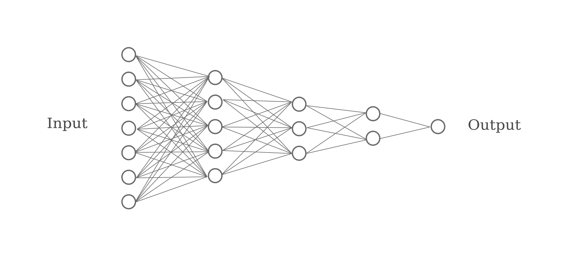
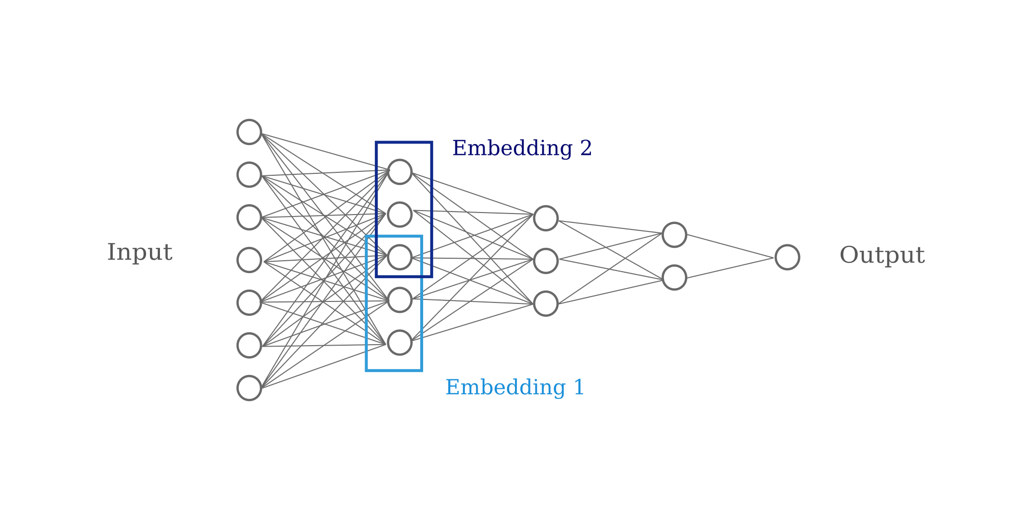
Consider the network architecture above: in this case the input is a tensor of concatenated one-hot vectors, and the output after three hidden layers is a single neuron that performs a linear regression on the second-to-last layer. Omitting most components, the architecture may be visualized as follows:

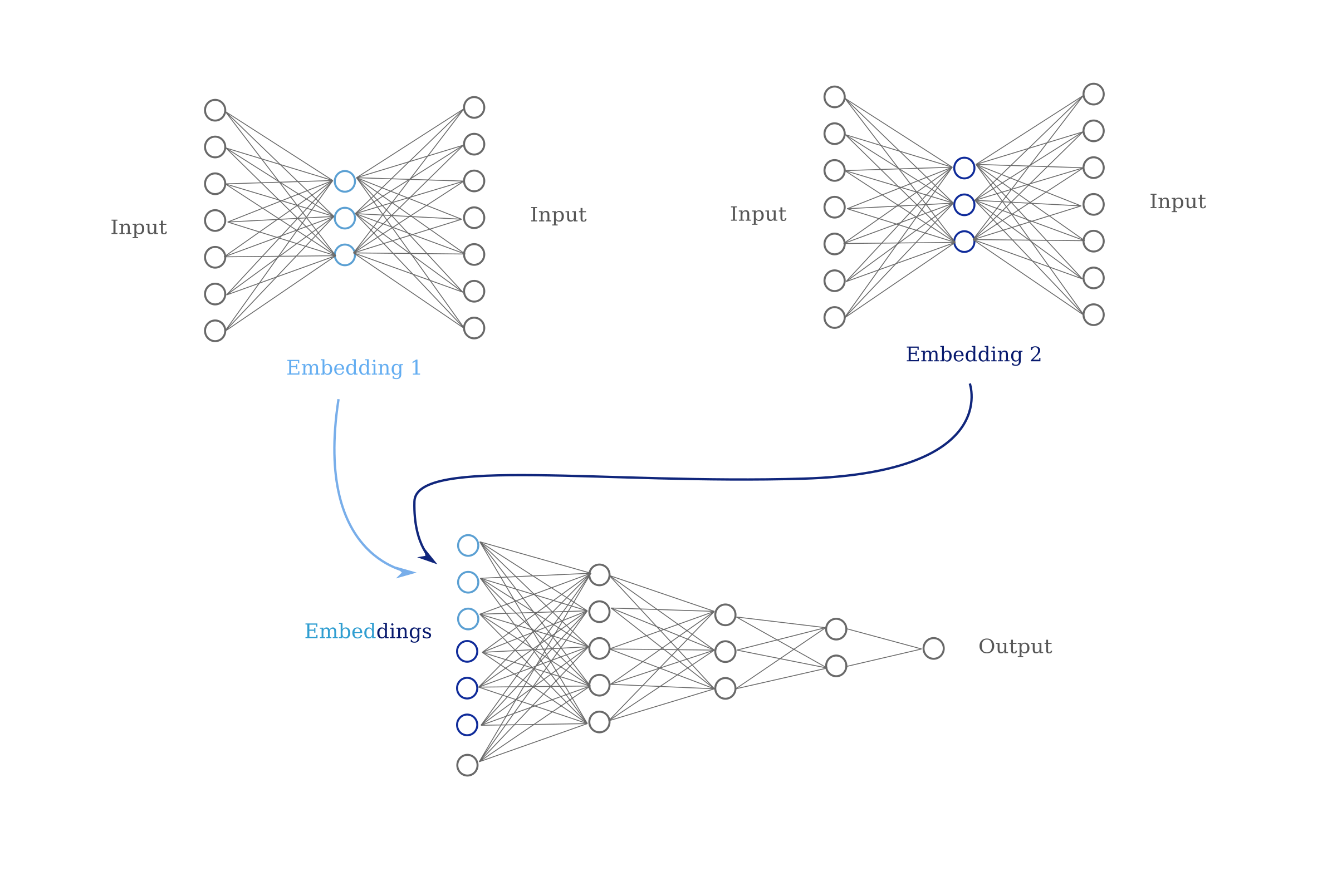
Now let’s compare this to the normal approach to encoding categorical inputs that may be of high dimensionality. Rather than employ large one-hot vectors, a better way is to perform embeddings on each of the features in question. This may be done with autoencoder neural networks as follows: first each feature is separated and then one hidden layer of smaller dimensionality than that input feature is trained to return the input as well as possible. The hidden layers contain what are normally called embeddings of the input.

Broadly speaking, an embedding is a structure-preserving map of one abstract object in another, for example the natural numbers in the integers. In the context of machine learning, embeddings are usually defined as vector spaces in which some distance metric of points in that space corresponds to a metric of those points outside the space in some significant measure. This means that more ‘similar’ examples (using some measure of significance to the machine learning task) will tend to be more ‘similar’, or in other words closer together, in the embedding. Useful embeddings are usually of lower dimension than the space of the inputs.

These hidden layers may then be used as the input layer of the deep learning model that will then produce an output. For a visualization of this process see below.

Consider what happens when we feed the input directly into the model, bypassing the embedding stage. If successful, each hidden layer of the model will learn one or more distributed representations of the input, meaning that the input will be represented accross each hidden layer such that the final representation allows for the final neuron to perform a linear regression $\hat {y} = w^Tx + b$ and obtain an accurate result, regardless of the true function one attempts to model.

In the model above, it is clear that each successive representation of the input will be of lower dimension than the last because each layer contains fewer parameters than the last. But in the general case, we can also say that between the input and output there is a representation that is of lower dimension than the input itself (otherwise training would be impossible, see the last section of this page for more details).

Containing input information in a space of smaller dimension than the input itself does not mean that deep learning models contain embeddings. But because we know that each layer is composed of a relatively simple continuous non-linear transformation of the prior layer, the second-to-last layer of an accurate deep learning model must be able to provide information necessary for the final layer to carry out its task with only one non-linear transformation. We know that the final layer’s vector space must reflect the measure of significance placed on the input, and therefore we can expect that the second-to-last layer’s vector space will also reflect this same measure of the input as most single non-linear used in deep learning applications transformations preserve relative distance.

Thus we are allowed to bypass an embedding stage because the model will be expected to obtain its own embeddings in each layer.

The traditional approach of first training embeddings using autoencoders before proceeding to use those as inputs into the model is analagous to greedy layer-wise pretraining for the first layer of the network, with the objective function being a distance measurement from the input rather than the model’s objective function.

Despite the theoretical reasons behind why an embedding would be expected to exist in a trained deep learning model, it may be wondered if there is any evidence for the claim that a feed-forward neural network learns a set of embeddings on the input. Happily we can simply use the (machine learning) definition of an embedding in order to test for the presence of this in a layer of a trained neural network.

Taking a trained version of the fully connected architecture shown in a previous section of this page, applied to the dataset with the output being a linear function of one input,

\[y=10d\]

we can test whether any layer forms an embedding on the inputs of this dataset by observing the correlation between the desired metric ($y$) for pairs of input examples versus some distance metric, say $L^1$, on the activations of a hidden layer. Choosing the last hidden layer, we have the following

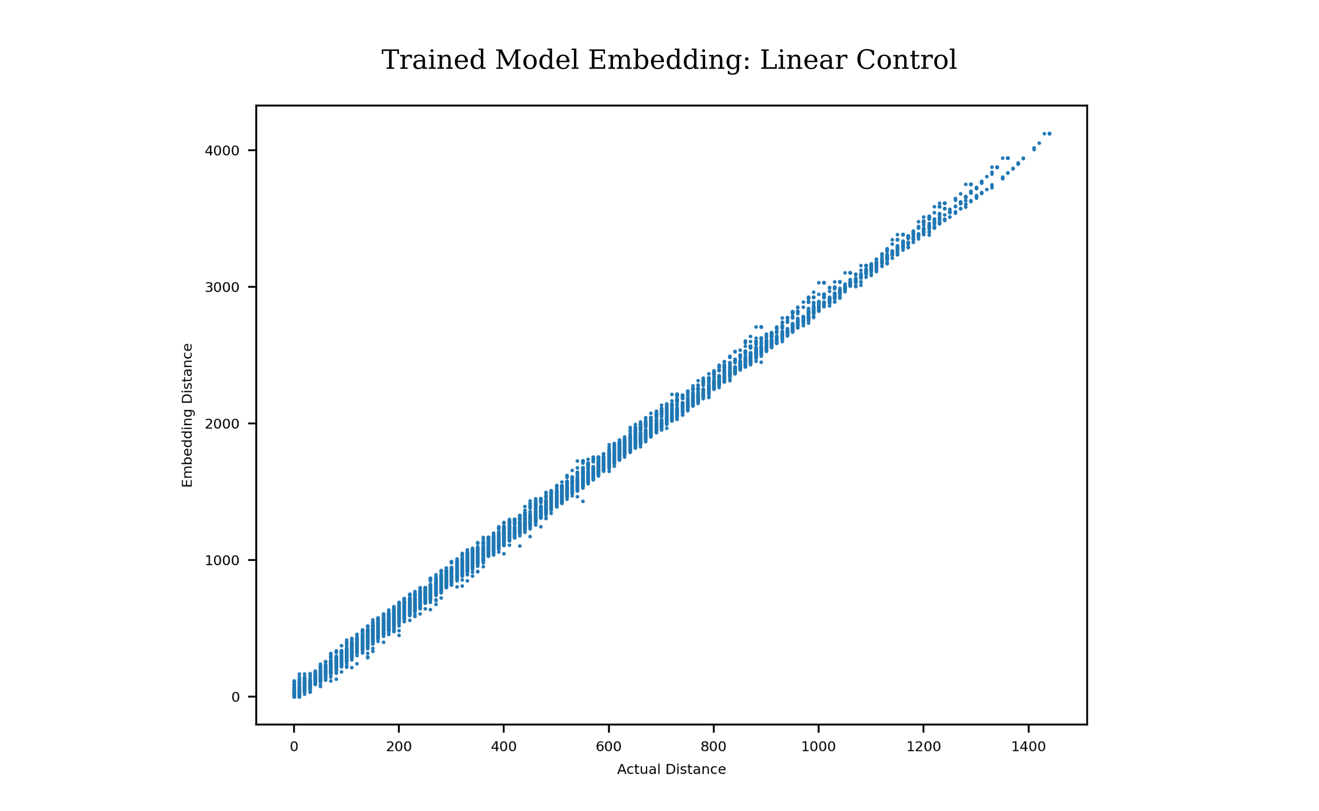
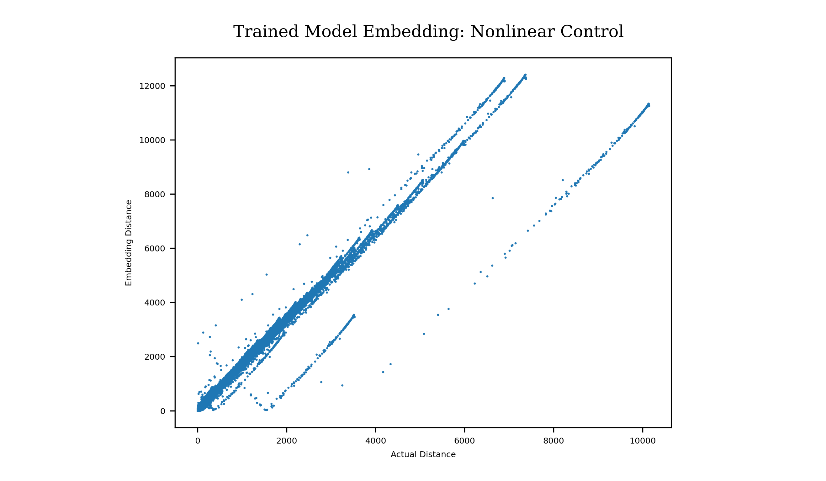
Thus we observe a correlation between the $l^1$ distance and the desired metric ($y$) and the final hidden layer for pairs of examples, which indicates that indeed the last hidden layer has formed a useful embedding on the input. We can also test whether the same model learns an embedding of the same inputs where the desired metric is

\[y = (c/100) * b\]

Before training, there is no correlation between pairs of examples in terms of actual distance versus embedding distance (both $L^1$ metric)

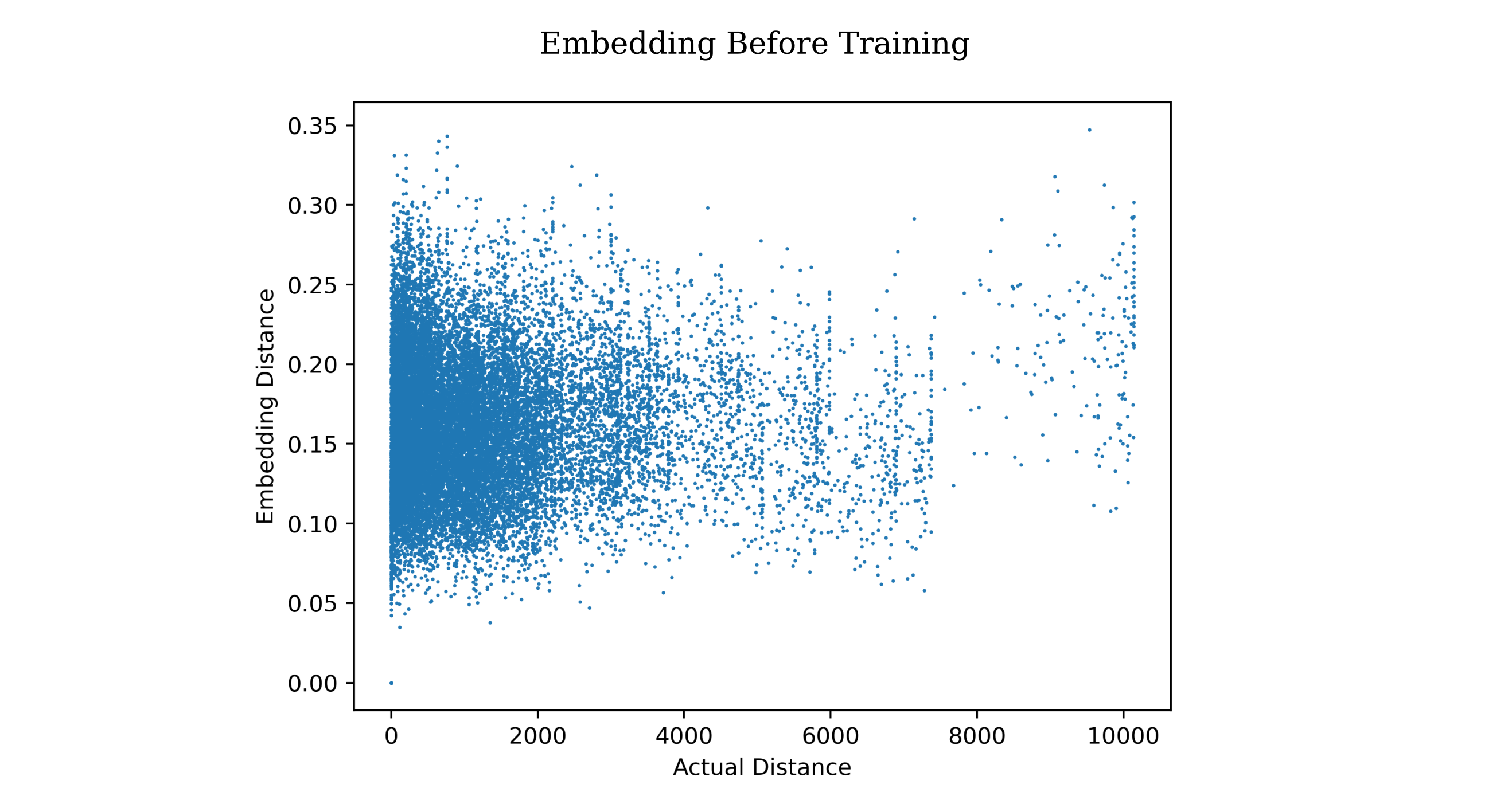
But after training, the correlation is found