Inherent limitations in neural nets

Neural networks can approximate only a subset of all functions

An oft-quoted feature of neural networks is that they are universal, meaning that they can compute any function (see here for a proof of this). A good geometrical explanation of this is found in Nielsen. Being that many everyday tasks can be thought of as some kind of function, and as neural networks are very good at a wide range of tasks (playing chess, recognizing images, language processing etc.) it can be tempting to see them as universal panacea for any problem. This view is mistaken, however, and to see why it is best to understand what exactly universality entails before exploring the limits of neural nets or any other similar approach.

There is an important qualification to the proof that neural networks can compute (more precisely, can arbitrarily approximate) any function: it only applies to continuous and differentiable functions. This means that neural networks should be capable of approximating any smooth and connected function, at least in theory. The first issue with this is whether or not a certain function is ‘trainable’, meaning whether or not a network is able to learn to approximate a function that is it theoretically capable of approximating. Putting this aside, the need for differentiability and continuity brings a far larger qualification to the statement of universality.

To see this, imagine that we were trying to use a neural network to compute an arbitrary function. What are the chances of this function being continuous and differentiable? Let’s see how many functions belong to one of three categories: differentiable (and continuous, as differentiability implies continuity), continuous but not necessarily differentiable, or not necessarily continuous or differentiable. Visually, differentiable functions are smooth with no sharp edges or squiggles and continuous functions may have sharp edges but must be connected.

Formally, we can define the set of all functions $f$ that map $X$ into $Y$, $f: X \to Y \; given \; X, Y \in \Bbb R$:

\[\{f \in (X, Y)\}\]

with the set of all continuous functions being

\[\{f \in \mathbf C(X, Y)\}\]

and the set of continuous and (somewhere) differentiable functions as

\[\{f \in \mathbf C^1(X, Y)\}\]

The cardinality of the set of all functions is equivalent to $ \Bbb R^{\Bbb R}$ and the cardinality of the set of all continuous functions is $\Bbb R$, so

\[\lvert \{f \in \mathbf C(X, Y)\} \rvert = \lvert \Bbb R \rvert << \lvert \Bbb R^{\Bbb R} \rvert = \lvert \{f \in (X, Y)\} \rvert\]

A small proof for this is as follows: continuous real functions map the real line onto the rationals and as the rationals are countable, the set of all continuous real functions is countable. In symbols,

\[\lvert \{f \in \mathbf C(X, Y)\} \rvert = \lvert \Bbb R ^ \Bbb Q \rvert = \lvert \Bbb R \rvert\]

Whereas real functions map the real line onto any point in this line (not necessarily rational points), so

\[\lvert \{f \in \mathbf (X, Y)\} \rvert = \lvert \Bbb R ^ \Bbb R \rvert\]

Set cardinality is intuitively a rather rough measure of the size of a set: the Cantor set, for example, has the same cardinality as $\Bbb R$ even though the probability of choosing an element in this set for all elements over the interval $[0, 1]$ is 0, and in that sense the Cantor set has a smaller measure than the reals.

More formally, as a consequence of Baire’s theorem, it can be shown that the set of somewhere-differentiable functions ${f \in \mathbf C^1(X, Y)}$ is of the first category (negligably small, specifically a union of countably many nowhere dense subsets) in Banach space (see Hewitt & Stromberg’s Real and Abstract analysis for a proof). Thus

\[m \{f \in \mathbf C^1(X, Y)\} << m \{f \in \mathbf C(X, Y)\}\]

where $m \mathbf C$ signifies the measure of the set of $ \mathbf C$. Expanding the definition of measure to be set cardinality inequality or Banach space inequality, we have:

\[m \{f \in \mathbf C^1(X, Y)\} << m \{f \in \mathbf C(X, Y)\} << m \{f \in (X, Y)\}\]

Thus size of the set of all continuous and differentiable functions is far smaller than the size of the set of all continuous functions, which is in turn far smaller than the set of all functions. The usage of ‘far smaller’ does not quite do justice to the idea that each set is vanishingly tiny compared to the next.

What does this mean? If we restrict ourselves to differentiable and continuous function then neural networks are indeed universal, but they are hardly so for all possible functions because differentiable and continuous functions are a tiny subset of all functions.

Limitations for all finite programs

Could it be that a better neural network will be made in the future, and this will allow us to compute nondifferentiable functions as well as differentiable ones? Using more concrete terms, perhaps we will be able to engineer a neural network that is arbitrarily precise at decision problems (which is equivalent to classification) in the future. This thinking can be used to represent the idea that although not perfect not, some sort of machine learning will be able to be arbitrarily good at decision making in the future. If not neural networks then perhaps decision trees: can some sort of machine learning program get so good at classification that it can learn how to classify anything, to arbitrary precision?

The answer is no: no matter what program we use, we cannot solve most decision problems. To see why, first note that any program, from a simple print (Hello World!) to a complicated neural network, is conveyed to a computer as a finite string of bits (a list of 1s and 0s). Natural numbers are also defined by a finite string of bits and so we can establish an equivalence between finite programs and natural numbers. The size of the set of all natural numbers is equivalent to the size of the set of all rational numbers (both are countably infinite).

\[\{\mathtt {finite} \; \mathtt {programs}\} = \{finite \; strings\; of\; bits\} \sim \Bbb N\]

A note on the precise symbols used here: $\sim$ indicates a set-theoretic equivalence relation, which means that there is a bijective (one-to-one and onto) mapping from one set to another, or informally that there are ‘as many’ elements in two sets. The equivalence relation $\sim$ is reflexive, transitive, and symmetric just like number theoretic equality $=$, but equivalence does not usually entail arbitrary replacement.

The size of the set of all natural numbers is equivalent to the size of the set of all rational numbers (both are countably infinite), so

\[\{\mathtt {finite} \; \mathtt {programs}\} \sim \Bbb N \sim \Bbb Q\]

Now let’s examine the set of all possible decision problems. We can restrict ourselves to binary classification without loss of generality, where we have two options: $1$ and $0$. Now a binary decision problem has an ouput 1 or 0 for every input, and we can list the outputs as a string of bits in binary point, ie binary digits that define a number between 0 and 1. As a decision problem must be defined for every possible input, and as there may be infinite inputs for any given decision problem, this string of bits is infinite and can define a number between 0 and 1.

\[\{decision\; problems\} = \{infinite \; strings\; of\; bits\} \sim \{x \in (0, 1]\}\]

As the size of the set of all numbers in $(0, 1]$ is equivalent to the size of the set of all real numbers,

\[\{decision \; problems\} \sim \Bbb R\]

and as the size of the set of all real numbers is uncountably infinite wheras the size of the set of all rational numbers is countably infinite,

\[\{decision \; problems\} \sim \Bbb R >> \Bbb Q \sim \{\mathtt {finite} \; \mathtt {programs}\}\]

This means that the set of all finite programs is a vanishingly small subset of the set of all decision problems, meaning that no finite program (or collection of programs) will ever be able to solve all decision problems, only a small subset of them.

Implications

The underlying point here is that there is a difference between strict universality in computer science and the idea of universality in functions. Universality in computer science is an idea that goes back to the Church-Turing thesis that any computable function may be evaluated by a certain machine, called a ‘Universal’ machine (Turing machines are a class of universal machines). Programming languages that are capable of defining procedures for all computable functions are termed ‘Turing complete’, and most general purpose languages that exist today are Turing complete.

Note that the class of computable functions extends far beyond the continuous, (piecewise) differentiable functions that have shown to be approximated by neural networks. But with more work, one can imagine that some future machine learning technique may approximate nondifferentiable and even discontinuous computable functions as well. Would that future machine learning program then be able to compute any function?

Not in the slightest: most functions are uncomputable. Specifically, if a random function were chosen then the probability that it is computable is 0. For why statement is true, see here. Now consider that functions describing the natural world are by no means computable. This means that there is no guarantee that the set of all computable functions (and therefore the set of all machine learning techniques in the future) will accurately describe the natural world in any way. For example, take the common physical constants $g$, $h$ etc. There is no evidence to suggest that any of these values are computable, or even rational. Even something as simple as a physical constant therefore is dubiously evaluated by a computable function.

Combining the observation that no program can help us evaluate an uncomputable expression with a consideration of what is computable and what is not, we can list a number of problems for which neural nets (or any machine learning procedure) are certainly incapable or not likely of assisting us:

1. Undecidable functions, such as the halting or total productivity problem: given a general recursive function (or Turing machine) with a certain number of states and inputs, determining whether the function ceases (or the machine halts), as well as what the greatest value possibly returned is, are both uncomputable and therefore unapproachable.

2. Undecidably-undecidable functions: attempting to prove the Goldbach conjecture, for example. This class of problem is not definately unapproachable via nets, but very likely is not.

3. Aperiodic long-term dynamical system behavior, such as the trajectories of three or more heavenly bodies or future iteration locations of the Henon attractor,

4. Natural processes that are best modelled by these aperiodic nonlinear dynamical equations are unlikely to be beneffited by nets or any other machine learning process. This category includes problems such as weather prediction, long-term stock market prediction, and turbulent flow trajectory determination.

All in all, a number of things that many people would want to predict or understand are either certainly or very probably incapable of being benefited by neural networks or any other sophistocated machine learning procedure. This includes fields like stock market prediction where attempts to predict using neural nets is underway.

A final note: the last section equated ‘arbitrary approximation’ with ‘equivalence’, in the sense that an arbitrary approximation of a function is the same as the function itself. But this is not true when the function is sensitive to initial conditions, because any error increases exponentially over time. In concrete terms, suppose one were to have a function that was in the rare computable category, and a neural net computed a close approximation of it. If that function described a non-linear change over time and the goal is long-term prediction, the network is not useful.

Neural networks as systems of dimension reduction: implications for adversarial examples

This section will explore an interesting consequence of precision in neural networks: adversarial examples, which are inputs that are nearly indistinguisheable from other inputs, the latter of which are accurately classified but the former are just as confidently mis-classified.

All supervised parametric statistical learning procedures, from linear regressions to neural networks, are subject to a bias-variance tradeoff. Test dataset classification errors are the result of irreducible error plus variance (sensitivity of the model to small changes in input) plus bias (error resulting from limitations in the chosen model) squared. Models that very restrictive assumptions (such as a linear regression) have high bias because such assumptions are rarely true even if they are convenient, whereas very flexible models like random forests or neural networks have lower bias as they make fewer restrictive assumptions but often exhibit higher variance, such that small changes to an input lead to large changes in output, whether that is a regression or else a classification as it is here. Adversarial examples can be viewed as examples of the effects of using models with high variance. Is this necessarily the case, or in other words can someone design a procedure that is of low bias but also free from effects of high variance?

Neural networks, like any statistical learning procedure, are in the business of dimensional reduction. This is because they take in inputs that are necessarily larger than outputs, which may seem counterintuitive if the inputs are small images and the outputs are choices between thousands of options. Even then, dimensional reduction holds: to see this, suppose that each image were classified into its own category. Then the network would not reduce dimension but the classification would be trivial: any program could do just as well by classifying any image to its own category. In the process of assigning multiple inputs to the same category, dimensional reduction occurs. To be specific, the many-dimensional training space is usually reduced to a one-dimensional cost function, and this is then used to change the network in order to decrease this cost function. This reduction is equivalent to a mapping, where one point in many dimensions is mapped to one corresponding point in one dimension.

As seen for the nonlinear attractors such as the one here, changes in dimension are not: small changes in inputs lead to large changes in attractor shape. Is a change in dimension always discontinuous? We are most interested here in a change from many dimensions to one, so start by considering the change in dimension from two to one.

The new question is as follows: can a mapping from a two dimensional surface to a one dimensional line be continuous? It turns out no: any mapping from two to one dimensions (with the mapping being one-to-one and onto) is discontinuous, to be specific it is everywhere discontinuous. Here ‘continuous’ as a property of functions is defined topologically as follows: in some metric space $(X, d)$ where $f$ maps to another metric space $(Y, d’)$, the function $f$ is continuous if and only if for any $\epsilon > 0$,

\[\lvert b - a \rvert < \delta \implies \lvert f(b) - f(a) \rvert < \epsilon\]

Where $\delta > 0$ is a distance in metric space $(X, d)$ and $\epsilon$ is a distance in metric space $(Y, d’)$. A discontinuous function is one where the above expression is not true for some pair $(a, b) \in X$ and an everywhere discontinous function is one in which the above expression is not true for every pair $(a, b) \in X$.

The statement is that any one-to-one and onto mapping from two dimensions to one is everywhere discontinuous. To show this we will make use of an elegant proof found in Pierce’s Introduction to Information Theory (p16-17).

Suppose we have arbitrary two points on a two dimensional surface, called $a$ and $b$. We can connect these points with an arbitrary curve, and now we choose two other points $c$ and $d$ on the surface and connect them with a curve that travels through the curve $ab$ as follows. All four points are mapped to a line, and in particular $a \to a’$, $b\to b’$ etc.

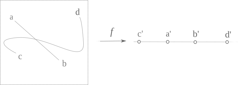
Now consider the intersection of $ab$ and $cd$. This intersection lies between $a’$ and $b’$ because it is on $ab$. But now note that all other points on $cd$ must lie outside $a’b’$ in order for this to be a one-to-one mapping. Thus there is some number $\delta > 0$ that exists separating the intersection point from the rest of the mapping of $cd$, and therefore the mapping is not continuous. To see that it is everywhere discontinous, observe that any point on the plane may be this intersection point, which maps to a discontinous region of the line. Therefore a one-to-one and onto mapping of a two dimensional plane to a one dimensional line is nowhere continuous $\square$.

This theorem also extends to the mappings of more than two dimensions to a line. If one reverses the direction of $f$ such that it maps a line to a plane (while keeping the one-to-one and onto stipulations), the theorem can also be extended to show that no bijective, continuous function can map a 1-dimensional line to a 2-dimensional surface. Plane-filling curves such as Peano or Hilbert curves (see here for more) are not continuous for a pre-image of finite size, and for either finite or infinite starting line lengths these curves are not one-to-one and are therefore not bijective.

Now consider the existence of adversarial examples, also called adversarial negatives, images that are by eye indistinguishable from each other but are seen by a network to be completely different. For some explanation of how these are generated and examples on images, see this article. The authors of this study suggest that the existence of these images suggests that the input-output mapping for a neural network is ‘fairly discontinuous’, and it is clear to see why: if two nearly-identical images are classified as very different, then two nearly-identical points in multidimensional input space end up being far from each other in output (and for a classification problem, therefore the predicted class).

Neural networks map many-dimensional space to one dimension, and as the proof above demonstrates this mapping must be discontinuous everywhere if the mapping is one-to-one, meaning that each different image has a different cost function associated with it. This means that every image classified by such a neural network will have an adversarial example, an image that is extremely close to one correctly classified but that will be incorrectly and confidently mis-classified.

Can we avoid discontinuous mapping when moving from two (or more) to one dimensions? Consider the following function

\[f:\Bbb R^2 \to \Bbb R\]

where

\[f(x_1, x_2) = x_1 + x_2\]

This mapping is continuous: arbitrarily small changes in the metric space $(\Bbb R^2, d)$ result in arbitrarily small changes in the corresponding slace $(\Bbb R, d’)$, and a sketch of a proof for this will be made apparent shortly.

How is this possible, given that one-to-one functions cannot map a surface to a line continuously? The above function is not one-to-one, instead an infinite number of starting points map to each point on $R$. To see why this is, consider which values of $a, b \; \lvert \; a \neq b$ are equal when mapped by $f$. Here $x_1 + x_2$ means adding coordinate values of the cartesian plane (ie $x$ value $+$ $y$ value). Which unique points on the plane would map to the same point on the real line using this function?

Consider $a = (0, 1)$ and $b = (1, 0)$. $f(a) = 1 = f(b)$, and indeed every point on the line $ab$ maps to the same value in $\Bbb R$, that is, $1$. Thus this function divides up $\Bbb R^2$ into diagonal lines, each line mapping to one point in $\Bbb R$. Now it should be easy to see why this function is continuous: it simply maps all points in $\Bbb R^2$ to the nearest position on the line $y = x$.

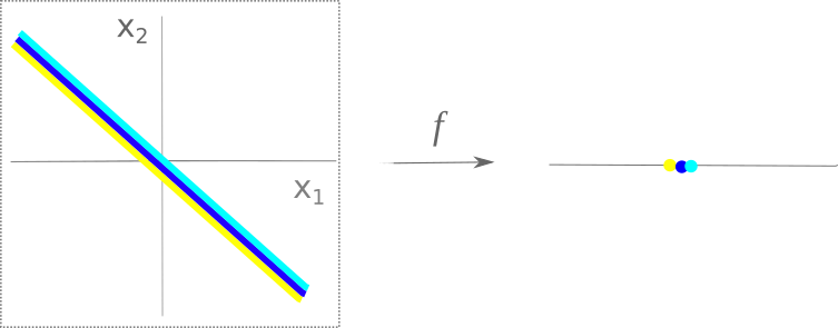
An arbitrarily small change perpendicular to this line in two dimensions yields no change in output in one dimension, and an arbitrarily small change applied along this line in two dimensions yields an arbitrarily small change in one dimension.

In sum, one-to-one (and onto) functions from two dimensions to one map discontinuously where as functions that are not one-to-one may map two dimensions to one continously. What does this mean for neural networks?

If we judge neural networks by their ability to classify an arbitrary number of input images into a finite number of outputs, it is clear that the neural network cannot act as a one-to-one function. But the process of training a network is as yet poorly achieved by using percent accuracy for a cost function, so the relevant output for the network is the (more or less) continuous cost function. With respect to this output, neural networks map each individual image to a specific value on the cost function and therefore act as a one-to-one mapping function during training. As training is what determines the final network function, a network trained using a continuous cost function acts as a one-to-one mapping between many dimensions and one.

In summary, neural networks that use a continuous cost function map (more than) two dimensions to one in a one-to-one mannar, and thus the mapping itself must be discontinuous (which results in adversarial negatives). Mappings that occur via discrete category selection are not one-to-one and therefore may be continuous, but such mappings are insufficient for training a network to be very precise. Thus it seems that the ability of a neural network (or any dimensional reduction machine learning technique) to learn to categorize precisely is inevitably connected with the appearance of adversarial examples, meaning that a precise network will have discontinuities in mapping regardless of how exactly the network is set up.

The implications of this are as follows: given any input and any neural net mapping inputs to a cost function in an (approximate) one-to-one manner, it is possible to find an adversarial example. To see why no input or network is safe, consider that the points $a$, $b$, $c$, and $d$ and the mapping funciton $f$ were chosen arbitrarily. Thus the finding that adversarial examples are inherent features of neural nets may be extended to any machine learning procedure that employs a near one-to-one mapping from input space to a cost function.

Why are adversarial examples relatively uncommon?

If adversarial examples follow from the fact that any mapping from $\Bbb R^n \to \Bbb R$ is everywhere discontinuous, why are adversarial examples not found everywhere? It is easy to see that adversarial examples must be rather rare, for otherwise training any network would be impossible. How can we reconcile the result that adversarial examples should occur wherever there is a discontinuity in mapping from $\Bbb R^n \to \Bbb R$ with the finding that in practice such examples are not common?

Machine learning methods relying on dimensional reduction (like deep learning via stochastic gradient descent) generally assume the the manifold hypothesis, which states that the probability distribution of relevant inputs (sound from speech, images of the natural world etc) are concentrated around low-dimensional manifolds in higher-dimensional space. For example, the following data points in two dimensional space are concentrated around a one-dimensional manifold denoted in blue:

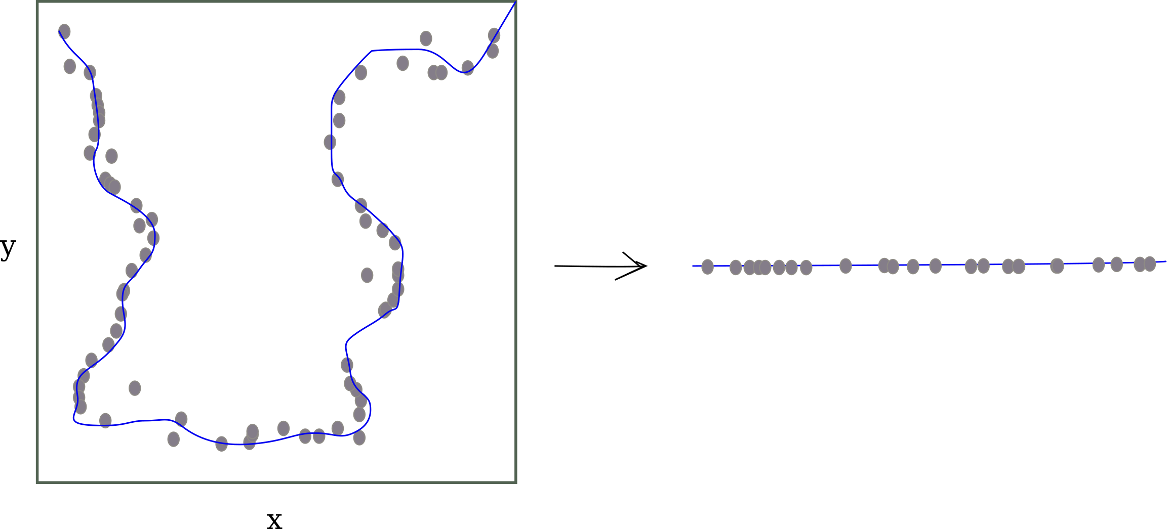
The manifold hypothesis requires two things to be true: first that inputs occupy very little (negligably small) of all possible input space, and second that all points sufficiently close together map to the same area on the lower dimensional manifold, not vastly separate regions.

It is clear that representations of relevant inputs are indeed only a small subset of all possible inputs: for example, most possible 20x20 images resemble noise rather than everyday objects. But while there is some experimental evidence for the second idea, the presence of adversarial negatives provides evidence against this idea as well leaving the overall accuracy of this statement ambiguous.

But then how are neural nets able to classify many inputs so effectively if we cannot assume the manifold hypothesis and furthermore if any one-to-one mapping from many dimensions to one is not continuous? Adversarial examples are generally of extremely low probability: if one simply adds noise with the same norm to an input before feeding that transformed input to a neural networks, a well-trained model typically does not exhibit large changes in output class estimation in nearly all cases. In other words, adversarial examples may be considered as exhibiting very low probability.

Another answer is that in practice one uses representations of multidimensional inputs and these representations are mappable bijectively with a one-dimensional encoded string (or integer, if one wants to think in those terms). In effect, no one has ever trained a network on a true multidimensional input because all current computational devices represent all inputs as one dimensional sequences of bytes. For example, the following 2-dimensional array could represent the information abc using one-hot vectors:

[[1, 0, 0, 0, ... 0],
 [0, 1, 0, 0, ... 0],
 [0, 0, 1, 0, ... 0]]

But this 2-dimensional array is only an abstraction for the programmer: the information is actually stored in memory by a 1-dimensional sequence of bits. This is accomplished because the following 1D array could be thought of as being equivalent to the 2D array above:

[1, 0, 0, 0, ... 0, 0, 1, 0, 0, ... 0, 0, 0, 1, 0, ... 0]

The same holds true of two-dimensional arrays corresponding to images of physical objects, of three-dimensional arrays representing time-series data, etc. And most importantly for this discussion, every input ever given to an artifical neural network is only a representation of a multidimensional input, an abstraction that is useful for thought but one that does not reflect the underlying 1D structure in memory. This means that every multidimensional object has already been bijectively mapped to a 1D object in the process of encoding, and therefore is not a true multidimensional object at all.

But then why do adversarial examples exist at all if neural nets simply map 1D arrays to other 1D arrays, which does not necessitate any discontinuity? This can be thought of as a result of increased resolution. As networks get more sophisticated and inputs take up more memory, the respresentations of both grow in size to become prodigiously large.

As input size increases, the input becomes more and more similar to a truly multidimensional object with respect to an output of fixed size (usually float or double), and the existance of adversarial examples becomes more common. This is why adversarial examples are relatively rare for small neural networks trained on low-information images (and why they have been found relatively recently in the history of machine learning research).