Diffusion Inversion Generative Models

An exploration of diffusion (aka denoising diffusion probabalistic) models.

Introduction with Denoising Autoencoders

Suppose one were to wonder how to de-noise an image that was corrupted some small amount. One way to approach this problem is to specify what exactly noise looks like such that it may be filtered out from an input. But if the type of noise were not known beforehand, it would not be possible to identify exactly what the noisy versus original parts of the corrupted image were. We therefore need some information on what the noise compared to the original image is, given samples of the original input $x$ and the corrupted samples $\widehat{x}$, it may be difficult to remove such noise in the general case.

As is often the case for poorly defined problems (in this case finding a general de-noiser), another way to address the problem of noise removal is to have a machine learning program learn how to accomplish noise removal in a probabalistic manner. A trained program would ideally be able to remove each element of noise with high likelihood.

One of the most effective ways of removing noise probabalistically is to use a deep learning model as the denoiser. Doing so allows us to refrain from specifying what the noise should look like, even in very general terms, which allows for a greater number of possible noise functions to be approximated by the model. Various loss functions may be used for the denoising autoencoder, one of which is Mean Squared Error (MSE),

\[L = || x - g(f(\widehat{x})) ||^2_2 \\ L = || x - g(h) ||^2_2\]

where $f(x)$ signifies the encoder which maps corrupted input $\widehat{x}$ to the hidden state $h$, also known as the ‘code’, and $g(h)$ maps this hidden state to the output.

In order to be able to successfully remove noise from an input, it is necessary for a model to learn something about the distribution of all uncorrupted inputs $p(x_i)$. Intuitively, the more a model is capable of recovering $p(x_i)$ the more it is capable of removing an arbitrary amount of noise.

Introduction to Diffusion Inversion

Now suppose that instead of recovering an input that has been corrupted slightly, we want instead to recover an input that was severely corrupted and is nearly indistinguisheable from noise. We could attempt to train our denoising autoencoder on samples with larger and larger amounts of noise, but doing so in most cases does not yield even a rough approximation of the desired input. This is because we are asking the autoencoder to perform a very difficult task because most images that one would want to reconstruct are really nothing like a typical noise sample at all.

The property that natural images are very different from noise is the motivation behind denoising diffusion models, also called denoising diffusion probabalistic modeling or simply diffusion models for short, originally introduced by Sohl-Dickinson and colleagues.

To make the very difficult task of removing a large amount of noise from a distribution approachable, we can break it into smaller sub-tasks that are more manageable. This is the same approach taken to optimiziation of any deep learning algorithm: finding a minimal value via a direct method is intractable, so instead we use gradient descent and the model will learn how many small steps towards a minimal point in the loss function space. Here we will teach a denoising autoencoder to remove both small and larger amount of noise from a corrupted input so that samples may be generated over many steps in order the reconstruct an input from pure noise.

Diffusion Theory

Diffusion inversion is defined on a forward diffusion process,

\[q(x_t | x_{t-1})\]

where $x_t$ signifies the input at time step $t$ in the diffusion process from 0 to the final time step $T$, ie $t \in {O, 1, … T}$. Therefore $x_0, x_1, …, x_T$ are latent variables of the same size as the input. This forward diffusion process is fixed and adds Gaussian noise at each step, such that for a fixed variance amount (known as a variance ‘schedule’) $\beta_t$ we can find the next forward diffusion step as follows:

\[q(x_t | x_{t-1}) = \mathcal {N}(x_t; \sqrt{1-\beta_t}x_{t-1}, \beta_t \mathbf(I))\]

The variance schedule is typically linear, with later work finding that a cosine schedule is sometimes more effective. Rather than compute $q(x_t \vert x_{t-1})$ by iterating the above equation the necessary number of times, there is happily a closed form

\[q(x_t | x_0) = \mathcal{N}(x_t; \sqrt{\bar \alpha_t}x_0, (1-\bar \alpha_t)\mathbf{I})\]

where $\alpha_t = 1 - \beta_t$ and $ \bar \alpha_t = \prod _ {s=1}^T \alpha_s$ is the cumulative variance by the end point $T$.

Inverting the diffusion process is equivalent to starting with pure noise $x_T$ and ending with a sample $x_0$.

\[p_{\theta} (x_0) = \int p(x_{0:T}) dx_{1:T}\]

With the (pure noise) starting point $x_T = \mathcal{N} (x_T; 0, I)$, a single step in the inverse diffusion process is as follows:

\[p_{\theta}(x_{t-1} | x_t) = \mathcal{N} \left ( x_{t-1}; \mu_{\theta} (x_t, t), \Sigma_{\theta}(x_t, t) \right )\]

Training the model $\theta$ involves estimating one (or more) of three quantities: the mean $\mu_{\theta} (x_t, t)$, variance $\mu_{\theta} (x_t, t)$, or else the Gaussian noise distribution $\epsilon \sim \mathcal{N}(0, I)$ which was introduced by Ho and colleagues. Ho and colleagues innovated by showing that superior empricial results could be obtained by training on a variant of the variational lower bound in which the model $\epsilon _ \theta$ attempts to learn the noise distribution $\epsilon$ via MSE loss,

\[L = || \epsilon - \epsilon_{\theta}(\sqrt{\bar \alpha_t}x_0 + \sqrt{1 - \bar \alpha_t}\epsilon, t)) ||_2^2\]

where $t$ is chosen to be uniform in $[1, T]$ and $T$ typically is on the order of 1000. The training process then consists of repeatedly sampling an input $x_0 \sim q(x_0)$ before choosing a time step $t$ and a Gausian distribution $\mathcal{N}(0, \mathbf{I})$ and then performing gradient descent on

\[\nabla_\theta || \epsilon - \epsilon_{\theta}(\sqrt{\bar \alpha_t}x_0 + \sqrt{1 - \bar \alpha_t}\epsilon, t)) ||_2^2\]

Here input images are expected to be scaled to have a minimum of -1 and maximum of 1 $x \in 0, 1, 2, …, 255 \to x \in [-1, 1]$. Ho and colleagues then re-weight $L$ to place more importance on larger corruptions (corresponding to larger $t$ values) reasoning that these would be more difficult for the model $\epsilon_\theta$ to learn than smaller corruptions.

To summarize, training a diffusion inversion model as presented by Ho and colleagues consists of teaching the model to predict the noise in a corrupted image, with the reasoning that after this occurs the model will be able to remove noise from a Gaussian distribution to generate new samples. Later work finds that switching between predicting $\epsilon$ and predicting $x_0$ leads to more effective training. THe model parameters $\theta$ are the same for all $t$ steps.

To generate samples, we want to learn the reverse diffusion process, $p_{\theta}(x_{t-1}, x_t)$. For diffusion inversion, this is the Markov chain where transitions are Gaussian distributions learned during the training process (which adds Gaussian distributions). Specifically, the input sampling process consists of first sampling the pure noise input $x_T \sim \mathcal{N}(0, \mathbf I) $ and then iterating for $t=T, T-1, …, 2$, first choosing noise $z \sim \mathcal{N}(0, \mathbf I) $ and then sampling

\[x_{t-1} = \frac{1}{\sqrt{\alpha_t}} \left( x_t - \frac{1 - \alpha_t}{\sqrt{1 - \bar \alpha_t}}\epsilon_\theta(x_t, t) \right) + \sigma_t z\]

Using Diffusion to generate handwritten digits

Let’s try to generate images of handwritten digits using diffusion inversion. First we need an autoencoder, and for that we can turn to a miniaturized and fully connected version of the well-known U-net architecture introduced by Ronnenberger and colleagues. The U-net architecture will be considered in more detail later, as for now we will make do with the fully connected version shown below:

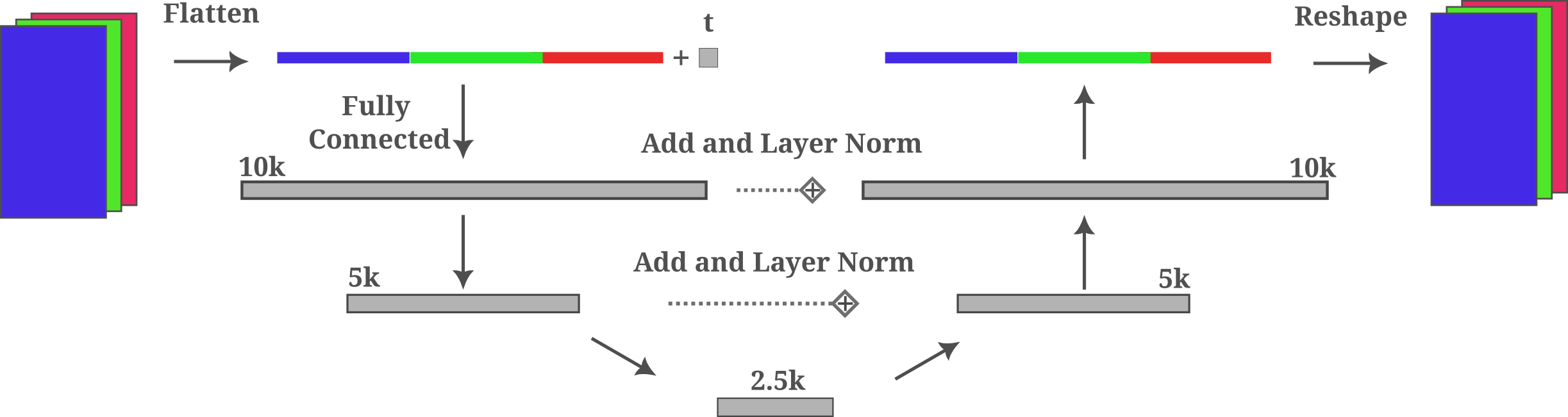
This is a variation of a typical undercomplete autoencoder which compresses the input somewhat (2k) using fully connected layers followed by de-compression where residual connections are added between layers of equal size, forming a distinctive U-shape. It should be noted that layer normalization may be ommitted without any noticeable effects. Layer sizes were determined upon some experimentation, where it was found that smaller (ie starting with 1k) widths trained very slowly.

Next we chose to take 1000 steps in the forward diffusion process, meaning that our model will learn to de-noise an input over 1k small steps in the diffusion inversion generative process as well. It is now necessary (for learning in a reasonable amount of time) to provide the time-step information to the model in some way: this allows the model to ‘know’ what time-step we are at and therefore approximately how much noise exists in the input. Ho and colleagues use positional encoding (inspired by the original transformer positional encodings for sequences) and therefore encode the time-step information as a trigonometric function added to the input (after a one-layer feedforward trainable layer). Although this approach would certainly be expected to be effective for a small model as well as large ones, we take the simpler approach of encoding time-step information in a single input element before appending that element to the others after flattening. Specifically, this time-step element $x_{t, n} = t / T$ where $t$ is the current time-step and $T$ is the final time-step.

An aside: it is interesting that time information is required for diffusion inversion at all, being that one might expect for an autoencoder trained to estimate the variance of the input noise relative to some slightly less-noisy input to be capable of estimating the accumulated noise as well, and therefore estimate the time-step value for itself. Removing the time-step information from the diffusion process of either the original U-net or the small autoencoder above yields poor sample generation but curiously the models are capable of optimizing the objective function without much trouble. It is currently unclear why time-step information is required for sample generation, ie $x_{T} \to x_{0}$, but not for minimizing $\epsilon - \epsilon(\sqrt \alpha_t x_0 + \sqrt{1 - \alpha_t}\epsilon)$.

Concatenation of a single element time-step value to the input tensor may be done as follows,

class FCEncoder(nn.Module):

	def __init__(self, starting_size, channels):
		super().__init__()
		starting = starting_size
		self.input_transform = nn.Linear(32*32*3 + 1, starting)
    ...

	def forward(self, input_tensor, time):
		time_tensor = torch.tensor(time/timesteps).reshape(batch_size, 1)
		input_tensor = torch.flatten(input_tensor, start_dim=1)
		input_tensor = torch.cat((input_tensor, time_tensor), dim=-1)
    ...

and the fully connected autoencoder combined with this one-element time information approach yields decent results after training on non-normalized MNIST data as shown below.

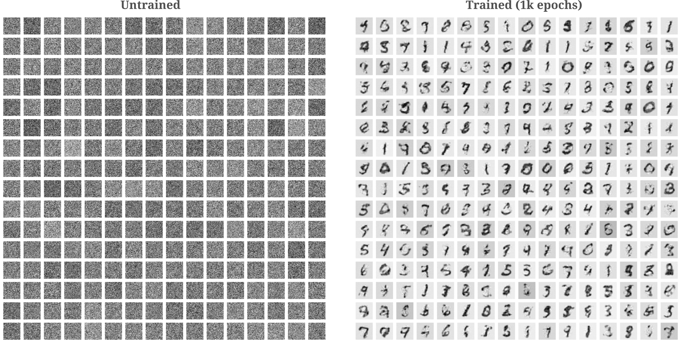
These results are somewhat more impressive when we consider that generative models typically struggle somewhat with un-normalized MNIST data, as most elements in the input are identically zero. Experimenting with different learning rates and input modifications convinces us that diffusion inversion is happily rather insensitive to exact parameter configurations, which is a marked difference from GAN training.

Attention Augmented Unet Diffision

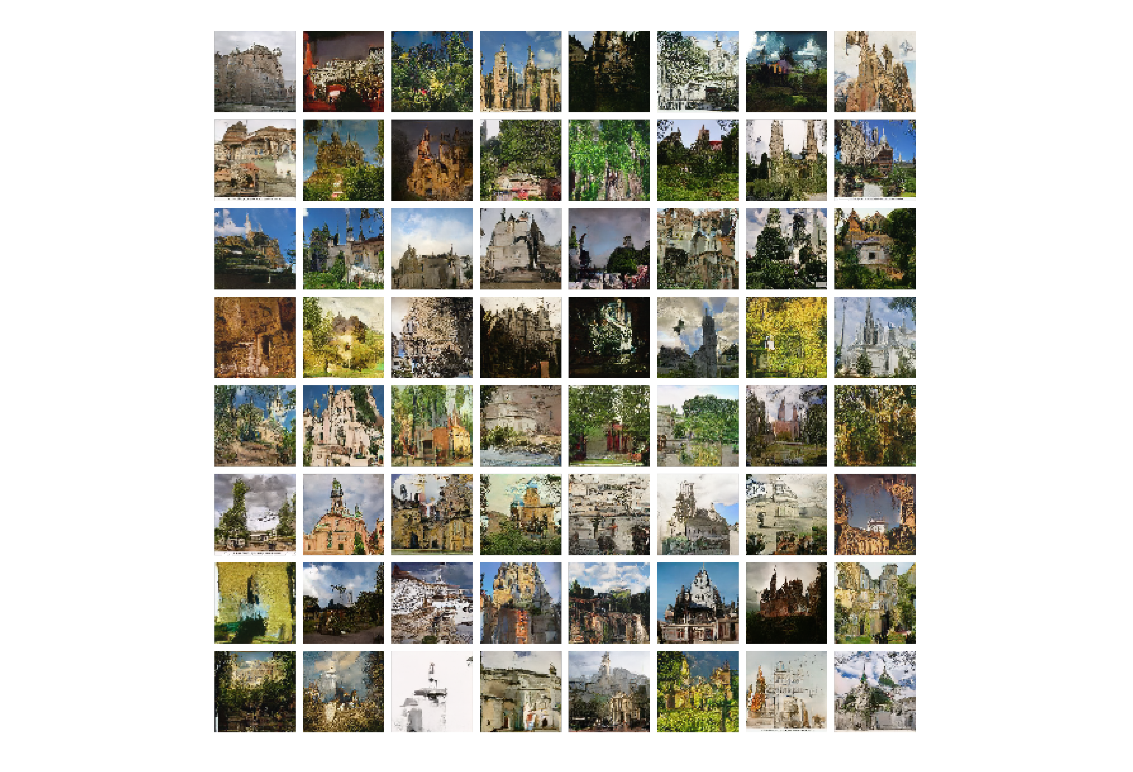
For higher-resolution images, the use of unmodified fully connected architectures is typically infeasible due to the very large number of parameters. Certain restrictions can be placed on the transformations between one layer and the next, and here we use both convolutions and attention in our denoising model to produce realistic images of churches.

We employ a modification on the original Unet architecture such that attention has been added at each layer, modified from Phil Wang’s implementation of the model introduced by Ho and colleagues. Here we use a four-deep Unet model with linear attention applied to residual connections and dot-product attention applied to the middle block. The general architecture is as follows:

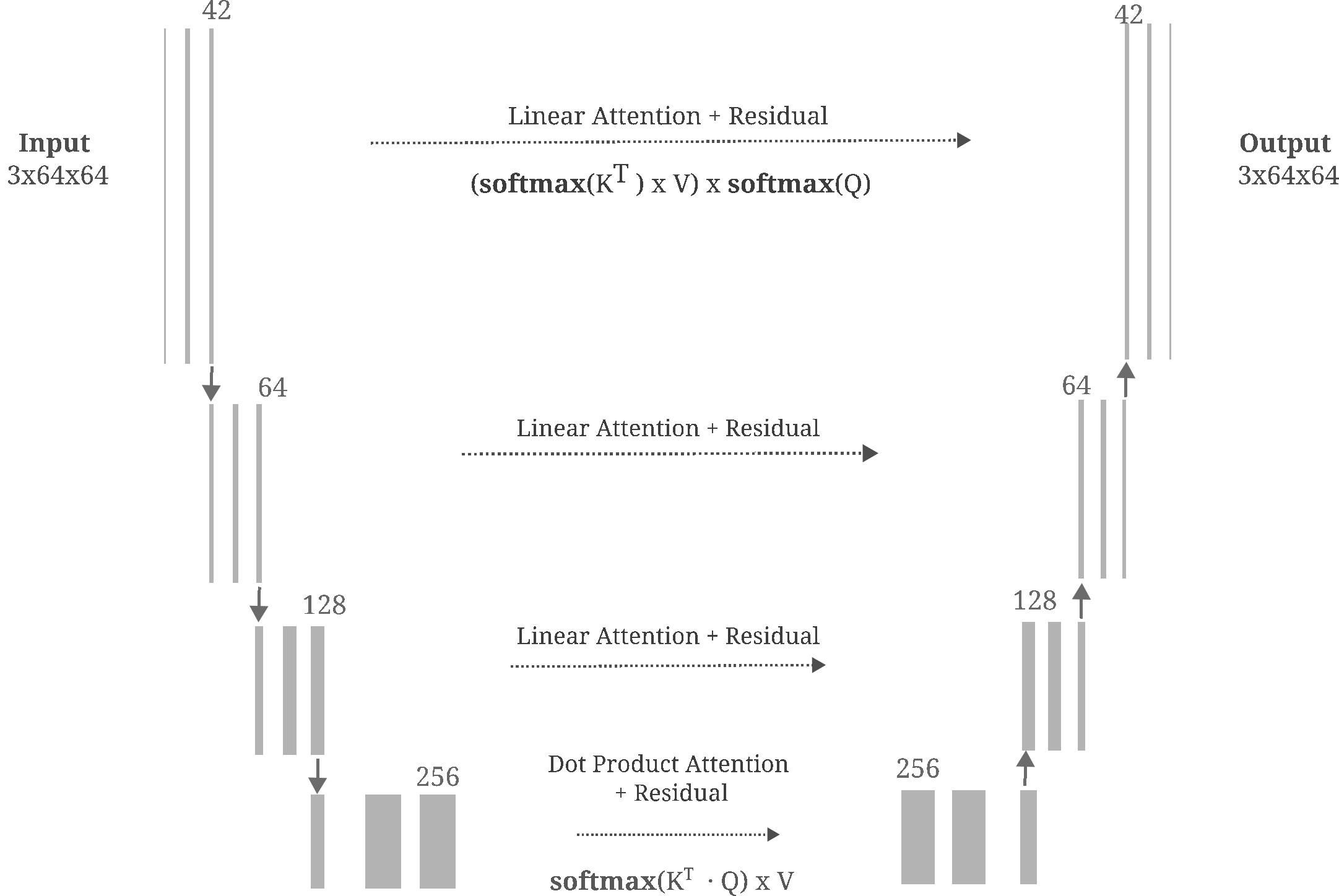
MLP activations for this model are Sigmoid Linear Units (SiLU)

\[f(x) = x * \sigma(x) = \frac{x}{1 + e^{-x}}\]

which is a very similar function to GeLU, and group norms are applied to each block and attention block (before the self-attention transformation). Time information is encoded into each blockvia a trainable MLP applied to fixed cosine-sine positional embeddings in the input. It is somewhat curious that this encoding of time into each block is beneficial, as positional encodings are usually applied only on the input.

After a couple hundred epochs of training on LSUN churches at $64^2$ resolution we have the following sampled images: