Generative Adversarial Networks

Introduction

Perhaps the primary challenge of using gradient descent on the input method for image generation (see here for more on this topic) is that the trained model in question was not tasked with generating inputs but with mapping them to outputs. With complicated ensembles composed of many nonlinear functions like neural networks, forward and reverse functions may behave quite differently. Instead of relying on our model trained for classification, it may be a better idea to directly train the model to generate images.

One method that takes this approach is the generative adversarial network model introduced by Goodfellow and colleages. This model used two neural networks that compete against each other (hence the term ‘adversarial’, which seems to have a different motivation than this term is used in the context of ‘adversarial examples’). One network, the discriminator, attempts to distinguish between real samples that come from a certain dataset and the generated samples that come from another network, appropriately named the generator. Theoretically, these two networks can compete against each other using the minimax algorithm to play a zero-sum game, although in practice GANs are implemented differently as minimax appears to be unstable in practice.

This method is of historical significance because it was a point of departure from other generative methods (Markov processes, inference networks etc.) that rely on averaging, either over the output space or the model parameter space. Generative adversarial networks generate samples with no averaging of either.

For discriminator model parameters $\theta_d$ and generator parameters $\theta_g$

\[f(d, g) = \mathrm{arg} \; \underset{g}{\mathrm{min}} \; \underset{d}{\mathrm{max}} \; v(\theta_d, \theta_g)\]

Following the zero-sum game, the minimax theorem posits that one player (the discriminator) wishes to maximize $v(\theta_d, \theta_g)$ and the other (in this case the generator) wishes to minimize $-v(\theta_d, \theta_g)$. We therefore want a value functions $v$ that grows as $d(x)$ becomes more accurate given samples $x$ taken from the data generating distribution $p(\mathrm{data})$ and shrinks (ie grows negatively) as $x$ is taken from outputs of the generator, denoted $p(\mathrm{model})$. One such option is as follows:

\[v(\theta_d, \theta_g) = \Bbb E_{x \sim p_{data}} \log d(x) + \Bbb E_{x \sim p_{model}} \log(1-d(x))\]

It is worth verifying that this value function does indeed satisfy our requirements. If we are given a set $x$ of only real examples $x \sim p_{data}$, $\Bbb E_{x \sim p_{model}} \log(1-d(x))$ can be disregarded as this is now an expectation over an empty set. A perfect discriminator would give classify all examples correctly, or $d(x) = 1$ making

\[\Bbb E_{x \sim p_{data}} \log d(x) = 0\]

As $d(x) \in [0, 1]$, it is clear that $v(\theta_d, \theta_g) \to 0$ as $d(x) \to 1$ and therefore $v$ increases to 0 from some negative starting point as the accuracy of $d(x)$ increases, meaning that the discriminator has maximized $v$.

Because of the log inverse function $\log(1-d(x))$ for the second term of $v(\theta_d, \theta_g)$, the opposite is true for the generator: if we assemble a dataset $x$ of examples only from the generator’s output, and if the generator was optimized at the expense of the discriminator, then the discriminator would predict the same output for the generated samples as for the real ones, or $d(x) = 1$. Therefore if the generator is optimized $d(g(x)) = 1$,

\[\Bbb E_{x \sim p_{model}} \log(1-d(x)) = \log(1 - 1) \\ = -\infty\]

then so too is $-v$ minimized, which was what we wanted.

The goal is for $g$ to converge to $g’$ such that $d(x) = 1/2$ for each input $x$ regardless of whether it was generated or not, which occurs when the generator emits inputs that are indistinguishable (for the discriminator) from the true dataset’s images.

Formulating the generative adversarial network in the form of the zero-sum minimax game above is the theoretical basis for GAN implementation. Unfortunately, this is a rather unstable arrangement because if we use $v$ and $-v$ as the payoff values, the generator’s gradient tends to vanish when the discriminator confidently rejects all generated inputs. During typical training runs this tends to happen, meaning that the desired state in which the discriminator neither rejects nor accepts all generated inputs is unstable. This does not mean that one could not train a GAN using a zero-sum minimax, but that choosing a value function that avoids instability is apparently rather difficult.

Goodfellow and colleages found that it is instead better to make the loss function of the generator equivalent to the log-probability that the discriminator has made mistake when attempting to classify images emitted from the generator, with a value (loss) function of binary cross-entropy for both discriminator and generator. The training process is no longer a zero-sum minimax game or even any other kind of minimax game, but instead is performed by alternating between minimization of cross-entropy loss of $d(x)$ for the discriminator and maximization of the cross-entropy loss of $d(g(z))$ for the generator, where $z$ signifies a random variable vector in the generator’s latent space.

The loss for the discrimator is binary cross-entropy between the predicted outputs, which are either 1 or 0 depending on if the discriminator thinks an image is real or fake,

\[d \in \{ y, 1-y \}\]

and actual labels,

\[q \in \{ \widehat y, 1 - \widehat y \}\]

which is denoted as

\[H(d, q) = -\sum_i d_i \log q_i \\ = -y \log \widehat y - (1-y) \log(1-\widehat y)\]

where $P(x)$ is equal to the distribution of $x$ over a mix of real and generated input and $Q(x)$ is the distribution of correct classifications of $P(x)$.

In contrast, the generator’s ojective is to fool the discriminator and so the target distribution $q’$ becomes $q’ = 1 - q \in {\widehat y, 1 - \widehat y}$, or in other words the generator uses the same binary cross-entropy applied to the discriminator but now with the labels reversed.

It is worth considering what this reformulation entails. For a single binary random variable, the Shannon self-entropy is as follows:

Implementing a GAN

The process of training a generative adversarial network may be thought of as consisting of many iterations of the two steps of our approximate minimax program above: first the discriminator is taught how to differentiate between real and generated images by applying the binary cross-entropy loss to a discriminator’s predictions for a set of generated samples and their labels followed by real samples and their labels,

def train_generative_adversaries(dataloader, discriminator, discriminator_optimizer, generator, generator_optimizer, loss_fn, epochs):
	discriminator.train()
	generator.train()

	for e in range(epochs):
		for batch, (x, y) in enumerate(dataloader):
			discriminator_optimizer.zero_grad()
			random_output = torch.randn(16, 5)
			
			generated_samples = generator(random_output)
			discriminator_prediction = discriminator(generated_samples)
			output_labels = torch.zeros(len(y), dtype=int) # generated examples have label 0
			discriminator_loss = loss_fn(discriminator_prediction, output_labels)
			discriminator_loss.backward()

			discriminator_prediction = discriminator(x)
			output_labels = torch.ones(len(y), dtype=int) # true examples have label 1
			discriminator_loss = loss_fn(discriminator_prediction, output_labels)
			discriminator_loss.backward() # add to previous loss
			discriminator_optimizer.step()

and then the generator is taught how to make images that fool the discriminator by finding the loss between the discriminator’s predictions for generated samples and a set of labels for real data.

			...
			generated_outputs = generator(random_output)
			discriminator_outputs = discriminator(generated_outputs)
			generator_loss = loss_fn(discriminator_outputs, torch.ones(len(y), dtype=int)) 
			
			generator_optimizer.zero_grad()
			generator_loss.backward()
			generator_optimizer.step()

The discriminator’s architecture is the same as any other network that maps $\Bbb R^n \to {0, 1}$. For a small image set such as the Fashion MNIST, we could have a multilayer perceptron with input of size 28*28=784, followed by a hidden layers and an output of size 1 as follows

class FCnet(nn.Module):

	def __init__(self):
		super().__init__()
		self.input_transform = nn.Linear(28*28, 1000)
		self.d1 = nn.Linear(1000, 400)
		self.d2 = nn.Linear(400, 200)
		self.d3 = nn.Linear(200, 1)
		self.relu = nn.ReLU()
		self.sigmoid = nn.Sigmoid()
		self.dropout = nn.Dropout(0.1)

	def forward(self, input_tensor):
		out = self.input_transform(input_tensor)
		out = self.relu(out)
		out = self.dropout(out)

		out = self.d1(out)
		out = self.relu(out)
		out = self.dropout(out)

		out = self.d2(out)
		out = self.relu(out)
		out = self.dropout(out)

		out = self.d3(out)
		out = self.sigmoid(out)
		return out

The generator may be a different architecture altogether, but here we can use an interted form of our MLP above. The latent space consists of 50 elements, which we will feed as 50 floating point numbers from a normal distribution.

class InvertedFC(nn.Module):

	def __init__(self):
		super().__init__()
		self.input_transform = nn.Linear(1000, 28*28)
		self.d3 = nn.Linear(400, 1000)
		self.d2 = nn.Linear(200, 400)
		self.d1 = nn.Linear(50, 200)
		self.relu = nn.ReLU()
		self.tanh= nn.Tanh()

	def forward(self, input_tensor):
		out = self.d1(input_tensor)
		out = self.relu(out)
		
		out = self.d2(out)
		out = self.relu(out)
		
		out = self.d3(out)
		out = self.relu(out)
		
		out = self.input_transform(out)
		out = self.tanh(out)
		return out

Using a latent space input of 100 random variables assigned in a normal distribution with $\sigma=1$ and $\mu=0$ followed by hidden layers of size 256, 512, and 1024 we find that the generator is able to produce images that are similar to the fashion mnist dataset. Here we observe a random sample of 100 latent space vectors over the training process (50 epochs)

Latent Space Exploration

Generative adversarial networks can go beyond simply producing images that look like they came from some real dataset: assuming that the relevant features of the input dataset’s distribution $p_{data}(x)$ have been captured by the generator, they can also be used to observe similarities in the inputs in a (usually) lower-dimensional tensor, the latent space. For the above video, each image is produced from 100 random numbers drawn from a normal distribution. If we change those numbers slightly, we might find changes in the output that lead to one image being transformed into another. In particular, the hope is that some low-dimensional transformation in the latent space yields a high-dimensional transformation in th egenerator’s output.

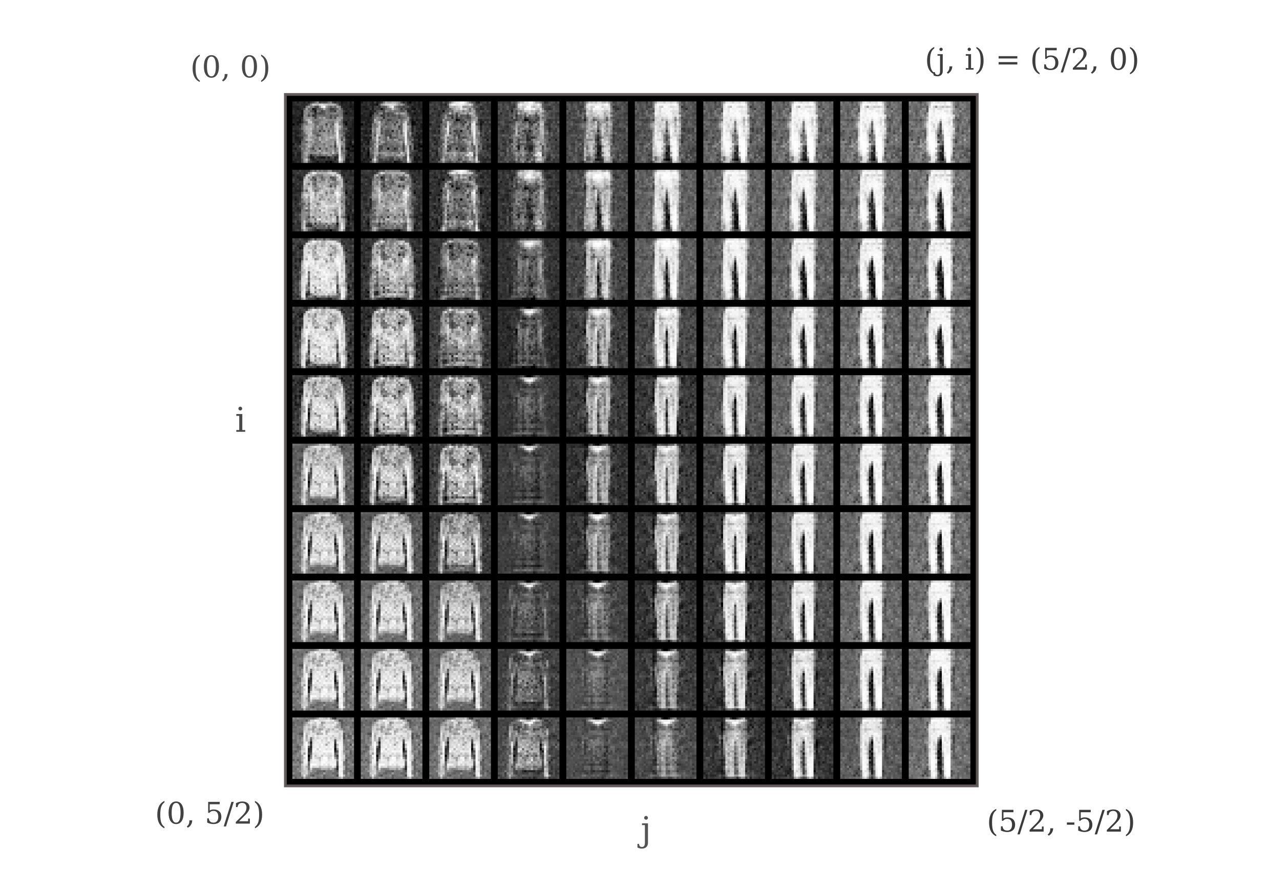
Somewhat surprisingly, this is indeed what we find: if move about in the latent space, the generated output changes fairly continuously from one clothing type to another. As an example, we can move through the 100-dimensional latent space in a 2-dimensional plane defined by simply adding or subtracting certain values from some random normal input. We can move in different ways, and one is as follows:

\[f(a, i, j) = a_{0:19} + i/4,\\ a_{20:39} - j/4, \\ a_{40:59} + i/4, \\ a_{60:79} - j/4, \\ a_{80:99} + j/4\]

which may be implemented as follows:

discriminator.load_state_dict(torch.load('discriminator.pth'))
generator.load_state_dict(torch.load('generator.pth'))

fixed_input = torch.randn(1, 100)
original_input = fixed_input.clone()

for i in range(10):
	for j in range(10):
		next_input = original_input.clone()
		next_input[0][0:20] += .25 * i
		next_input[0][20:40] -= .25 * j
		next_input[0][40:60] += .25 * i
		next_input[0][60:80] -= .25 * j
		next_input[0][80:100] += .25 * j
		fixed_input = torch.cat([fixed_input, next_input])

fixed_input = fixed_input[1:]
output = generator(fixed_input)
output = output.reshape(100, 28, 28).cpu().detach().numpy()

when we observe the elements of output arranged such that the y-axis corresponds to increass in i and the x-axis (horizontal) corresponds to increases in j, we have the following:

Does manifold learning occur for generative adversarial networks trained on other datasets? We can apply our model to the MNIST handwritted digit dataset by loading the training data

train_data = torchvision.datasets.MNIST(
	root = '.',
	train = True,
	transform = tensorify_and_normalize,
  	download = True
	)

Now most images in the MNIST dataset contain lots of blank space, meaning that for a typical input most tensor elements are 0s. This make GAN learning difficult, so it is a good idea to enforce a non-zero mean on our inputs. One option that seems to work well is to set the mean $\mu$ and standard deviation $\sigma$ to be given values by performing the following element-wise operation

\[a_i = \frac{a_i - \mu}{\sigma}\]

and this can be implemented using torchvision.transforms as follows:

tensorify_and_normalize = transforms.Compose(
    [transforms.ToTensor(), transforms.Normalize((0.5), (0.5))]
)

In the last illustration, we moved through 100-dimensional space along a 2-dimensional hyperplane to observe the latent space manifold. This makes it somewhat confusing to visualize, so instead we can simply begin with a 2-dimensional manifold as our latent space, with a generator architecture as follows:

class InvertedFC(nn.Module):
	def __init__(self):
		super().__init__()
		self.input_transform = nn.Linear(1024, 28*28)
		self.d3 = nn.Linear(512, 1024)
		self.d2 = nn.Linear(248, 512)
		self.d1 = nn.Linear(2, 248)
		...

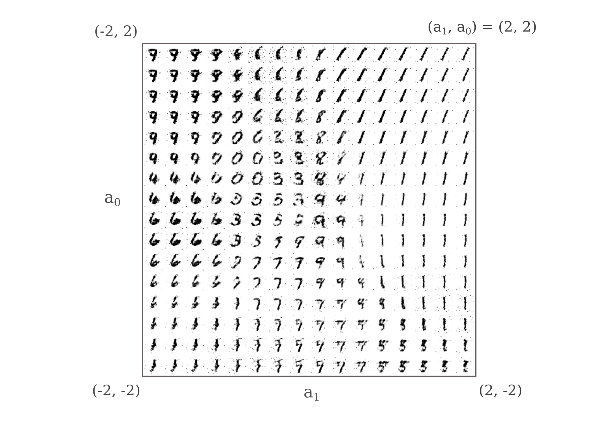
Now that the latent space is two-dimensional, we can observe the manifold more clearly in a plane. As generator latent space inputs are random normal variables ($\mu=0$, $\sigma=1$), we know most of the inputs are in near the origin. Tracing out a square from (-2, -2) to (2, 2)

discriminator.load_state_dict(torch.load('discriminator.pth'))
generator.load_state_dict(torch.load('generator.pth'))
fixed_input = torch.tensor([[0.,  0.]]).to(device)
original_input = fixed_input.clone()

for i in range(16):
  for j in range(16):
    next_input = original_input.clone()
    next_input[0][0] = 2 - (1/4) * (i) + original_input[0][0]
    next_input[0][1] = -2 + (1/4) * (j) + original_input[0][1]
    fixed_input = torch.cat([fixed_input, next_input])

fixed_input = fixed_input[1:]

we see that indeed nearly every digit is found in this region of the latent space, as expected.

We can perform the same procedure for the Fashion MNIST dataset by training a GAN with a latent space of size 2.

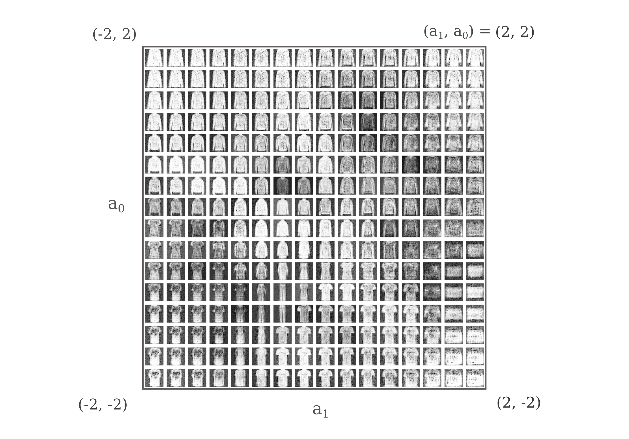
Do generative adversarial networks tend to prefer a stereotypical generator configuration $\theta_s$ on the latent space over other possible configurations? To be concrete, do GANs of one particular architecture when trained repeatedly on the same dataset tend to generate the same images for a given coordinate $a_1, a_2, …, a_n$ in the latent space? Visualization is often difficult for a high-dimensional latent space, but is perfectly approachable in two dimensions. We can therefore design a GAN with a two-dimensional latent space as has been done above and observe whether or not the same generated images are found at any given coordinate for multiple training runs. The answer is no, for any coordinate $a_n$ in latent space we do not find a similar generated image from one training run to the next.

Continuity and GAN stability

It is interesting to observe how relatively difficult it is to train a GAN, especially compared to the process of training an image classification model alone.

Unstable Convolutional GANs

For large images, fully connected network GANs become less practical due to the exponential number of trainable parameters in both generator and discriminator. Convolutional neural networks generally perform very well at object recognition tasks, and so it is natural to wonder whether they would also make effective generative networks too.

Convolutional neural networks have been historically viewed as difficult to use as discriminator/generator pairs in the GAN model. Empirically this has been attributed to their tendancy to lead to instabilities while training: either the discriminator may become much more effective than the generator such that all generated inputs are confidently rejected, or else the generator may be able to fool the discriminator early in the training program, which reduces the objective gradient for the discriminator and thus prevents effective learning.

Some of the difficult stems from the nature of the convolution, which as defined in the context of deep learning signifies a mathematical function on tensors of real numbers that is strictly non-invertable as it is non-injective. To see why this is, take the simple example of a convolution on a two-element array of one dimension, with a kernal of $\gamma= [\gamma_1, \gamma_2]$ and no padding:

\[f([a, b], \gamma) = a \gamma_1 + b \gamma_2 = c\]

Is there any way, if one knows $c$ and $\gamma$ to compute $[a, b]$? There is not, as different values of $a, b$ would give equivalent values of $c$ and thus this function is not injective. More precisely, any linear combination of $a + b = c$ will suffice.

This is important because it means that there is no way to unambiguously invert a convolutional discriminator architecture. We could of course use a convolutional net for a discriminator and a fully connected architecture for the generator, but doing so risks the instabilities mentioned above.

In spite of these challenges, we can go ahead and implement a convolutional GAN to see how it performs. For the discriminator, we can use the same architecure used elsewhere on this page for classifying flower types, with two notable changes: firstly, dropout is introduced to the fully connected layers and secondly we now store the indices identified by the max pooling steps (which signifies the indices of the elements that contributes their values to the subsequent pooling layer). Max pooling by itself non-injective and thus non-invertible function, and using the indicies of the discriminator is one way to allow make max pooling invertible.

class MediumNetwork(nn.Module):

	def __init__(self):
		super(MediumNetwork, self).__init__()
		self.entry_conv = Conv2d(3, 16, 3, padding=(1, 1))
		self.conv16 = Conv2d(16, 16, 3, padding=(1, 1))
		self.conv32 = Conv2d(16, 32, 3, padding=(1, 1))

		self.max_pooling = nn.MaxPool2d(2, return_indices=True)
		self.flatten = nn.Flatten()
		self.relu = nn.ReLU()
		self.d1 = nn.Linear(2048, 512)
		self.d2 = nn.Linear(512, 50)
		self.d3 = nn.Linear(50, 1)
		self.sigmoid = nn.Sigmoid()
		self.dropout = nn.Dropout(0.1)
		self.index1, self.index2, self.index3, self.index4 = [], [], [], [] # save indicies for max unpooling in generator
		
	def forward(self, model_input):
		out = self.relu(self.entry_conv(model_input))
		out, self.index1 = self.max_pooling(out)
		out = self.relu(self.conv16(out))
		out, self.index2 = self.max_pooling(out)
		out = self.relu(self.conv16(out))
		out, self.index3 = self.max_pooling(out)
		out = self.relu(self.conv32(out))
		out, self.index4 = self.max_pooling(out)
		output = torch.flatten(out, 1, 3)

		output = self.d1(output)
		output = self.relu(output)
		output = self.dropout(output)

		output = self.d2(output)
		output = self.relu(output)
		output = self.dropout(output)

		final_output = self.d3(output)
		final_output = self.sigmoid(final_output)
		return final_output

Now we can make essentially the same architecture in reverse, but starting with a latent space of size 50. The model below uses the max pooling indicies obtained by the discriminator at each step of the training process, which is a somewhat dubious choice as doing so has the potential to bring about memorization of the training set.

class InvertedMediumNet(nn.Module):

	def __init__(self, minibatch_size):
		super(InvertedMediumNet, self).__init__()
		self.entry_conv = Conv2d(16, 3, 3, padding=(1, 1))
		self.conv16 = Conv2d(16, 16, 3, padding=(1, 1))
		self.conv32 = Conv2d(32, 16, 3, padding=(1, 1))

		self.max_pooling = nn.MaxUnpool2d(2)
		self.minibatch_size
		self.relu = nn.ReLU()
		self.tanh = nn.Tanh()
		self.d1 = nn.Linear(512, 2048)
		self.d2 = nn.Linear(50, 512)

	def forward(self, final_output):
		output = self.d2(final_output)
		output = self.relu(output)
		output = self.d1(output)
		output = self.relu(output)

		out = torch.reshape(output, (self.minibatch_size, 32, 8, 8)) # reshape for convolutions
		out = self.max_pooling(out, discriminator.index4)
		out = self.relu(self.conv32(out))
		out = self.max_pooling(out, discriminator.index3)
		out = self.relu(self.conv16(out))
		out = self.max_pooling(out, discriminator.index2)
		out = self.relu(self.conv16(out))
		out = self.max_pooling(out, discriminator.index1)
		out = self.tanh(self.entry_conv(out))
		return out

In practice, however, the use of an input’s max pooling indicies appears to not result in memorization a sigmoid unit discriminator output is combined with binary cross-entropy. If a softmax output layer is used instead, weak memorization early in the training process has been observed. If memorization is suspected to become a problem, it is not difficult to avoid the issue of transfer of max pooling indicies by either fixing them in place or else using the pooling indicies of a the discriminator applied to a generated example rather than a true input.

The training proceeds the same way as the other GAN examples, except we need to initialize the generator’s max unpooling indicies. Below the indicies from the discrimantor applied to the input tensor x are used for initialization.

def train_colorgan_adversaries(dataloader, discriminator, discriminator_optimizer, generator, generator_optimizer, loss_fn):
	fixed_input = torch.randn(minibatch_size, 50) # latent space of 50
	for batch, (x, y) in enumerate(dataloader):
		count += 1
		_ = discriminator(x) # initialize the index arrays
		random_output = torch.randn(minibatch_size, 50).to(device)
		generated_samples = generator(random_output)
		...

This method is at least somewhat successful: comparing six training input images to six generated inputs from our flower identification dataset, we see there is some general resemblance between the generated data and the original.

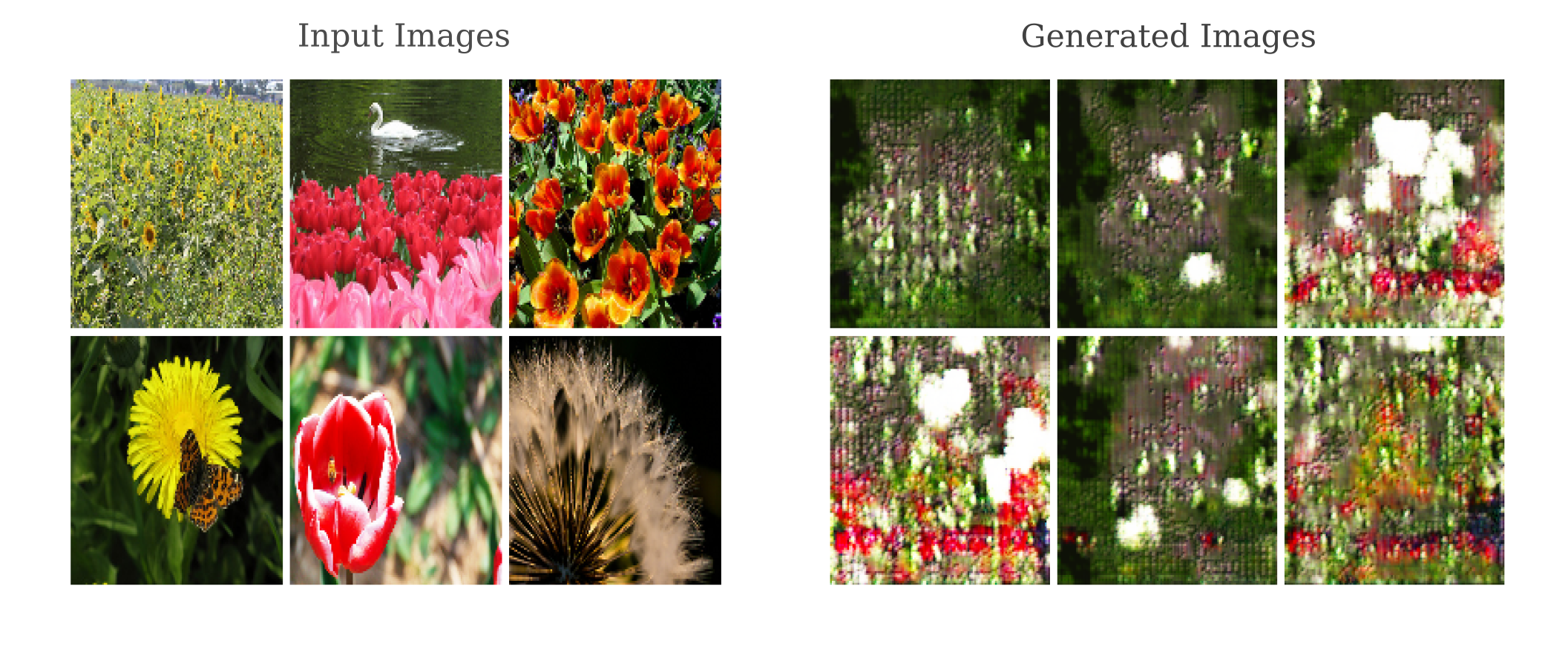
But unfortunately this architecture tends to be unstable while training, and in particular the generator seems to be often incapable of producing images that challenge the discriminator’s ability to discern them from the real inputs.

Semi Stable Convolutional GANs

Difficulties with generative adversarial networks based on deep convolutional networks were well documented in the early days of research into GANs. One approach to working around this problem is that taken by Radford and colleagues. They detail a model architecture in which both generator and discriminator are composed entirely of convolutional layers as opposed to a mixture of convolutional and fully connected hidden layers, batch normalization is used for both generator and discriminator hidden layers, and unpooling is replaced with fractional convolutional layers. The architecture published in the paper above is now referred to as ‘DCGAN’, id deep convolutional GAN.

Using these principles, we can make a DCGAN-like discriminator that takes 3x128x128 color images as inputs and returns a sigmoid transformation with image $y\in(0, 1)$ which corresponds to whether or not a given image is one from our training dataset.

class StableDiscriminator(nn.Module):

	def __init__(self):
		super(StableDiscriminator, self).__init__()
		# switch second index to 3 for color
		self.conv1 = nn.Conv2d(3, 64, 4, stride=2, padding=1) # 3x128x128 image input
		self.conv2 = nn.Conv2d(64, 128, 4, stride=2, padding=1)
		self.conv3 = nn.Conv2d(128, 256, 4, stride=2, padding=1)
		self.conv4 = nn.Conv2d(256, 512, 4, stride=2, padding=1)
		self.conv5 = nn.Conv2d(512, 1024, 4, stride=2, padding=1)
		self.conv6 = nn.Conv2d(1024, 1, 4, stride=1, padding=0)

		self.leakyrelu = nn.LeakyReLU(negative_slope=0.2)
		self.batchnorm2 = nn.BatchNorm2d(128)
		self.batchnorm3 = nn.BatchNorm2d(256)
		self.batchnorm4 = nn.BatchNorm2d(512)
		self.batchnorm5 = nn.BatchNorm2d(1024)
		self.sigmoid = nn.Sigmoid()

	def forward(self, input):
		out = self.conv1(input)
		out = self.leakyrelu(out)
		
		out = self.conv2(out)
		out = self.leakyrelu(out)
		out = self.batchnorm2(out)
		
		out = self.conv3(out)
		out = self.leakyrelu(out)
		out = self.batchnorm3(out)
		
		out = self.conv4(out)
		out = self.leakyrelu(out)
		out = self.batchnorm4(out)
		
		out = self.conv5(out)
		out = self.leakyrelu(out)
		out = self.batchnorm5(out)
		
		out = self.conv6(out)
		out = self.sigmoid(out)
		return out

For the generator again we follow the original DCGAN layer dimensions fairly closely, but deviate in a couple key areas to allow for a 100-dimensional latent space input to give a 3x128x128 generated image output. Note that in the original paper, the exact choice of transformation between the input layer and the first convolutional layer is somewhat ambiguous: either a fully connected layer (with no activation function) or else a direct reshape and projection are potential implementations. We take the latter approach (also taken here) as the former tends to lead to the problem of diminishing gradients that convolutional netowrks with deep fully connected hidden layers seem to face.

class StableGenerator(nn.Module):

	def __init__(self, minibatch_size):
		super(StableGenerator, self).__init__()
		self.input_transform = nn.ConvTranspose2d(100, 1024, 4, 1, padding=0) # expects an input of shape 1x100
		self.conv1 = nn.ConvTranspose2d(1024, 512, 4, stride=2, padding=1) 
		self.conv2 = nn.ConvTranspose2d(512, 256, 4, stride=2, padding=1)
		self.conv3 = nn.ConvTranspose2d(256, 128, 4, stride=2, padding=1)
		self.conv4 = nn.ConvTranspose2d(128, 64, 4, stride=2, padding=1)
		self.conv5 = nn.ConvTranspose2d(64, 3, 4, stride=2, padding=1) # end with shape minibatch_sizex3x128x128

		self.relu = nn.ReLU()
		self.tanh = nn.Tanh()
		self.minibatch_size = minibatch_size
		self.batchnorm1 = nn.BatchNorm2d(512)
		self.batchnorm2 = nn.BatchNorm2d(256)
		self.batchnorm3 = nn.BatchNorm2d(128)
		self.batchnorm4 = nn.BatchNorm2d(64)

	def forward(self, input):
		input = input.reshape(minibatch_size, 100, 1, 1)
		transformed_input = self.input_transform(input)
		out = self.conv1(transformed_input)
		out = self.relu(out)
		out = self.batchnorm1(out)
		
		out = self.conv2(out)
		out = self.relu(out)
		out = self.batchnorm2(out)
		
		out = self.conv3(out)
		out = self.relu(out)
		out = self.batchnorm3(out)
		
		out = self.conv4(out)
		out = self.relu(out)
		out = self.batchnorm4(out)
		
		out = self.conv5(out)
		out = self.tanh(out)
		return out

Lastly, our original flower image dataset contained a wide array of images (some of which did not contain any flowers at all), making generative learning difficult. A small (n=249) subset of rose and tulip flower images were selected for training using the DCGAN -style model. This small dataset brings its own challenges, as deep learning in general tends to be easier with larger sample sizes.

The results are fairly realistic-looking, and some generated images have a marked similarity to watercolor images of roses or tulips.

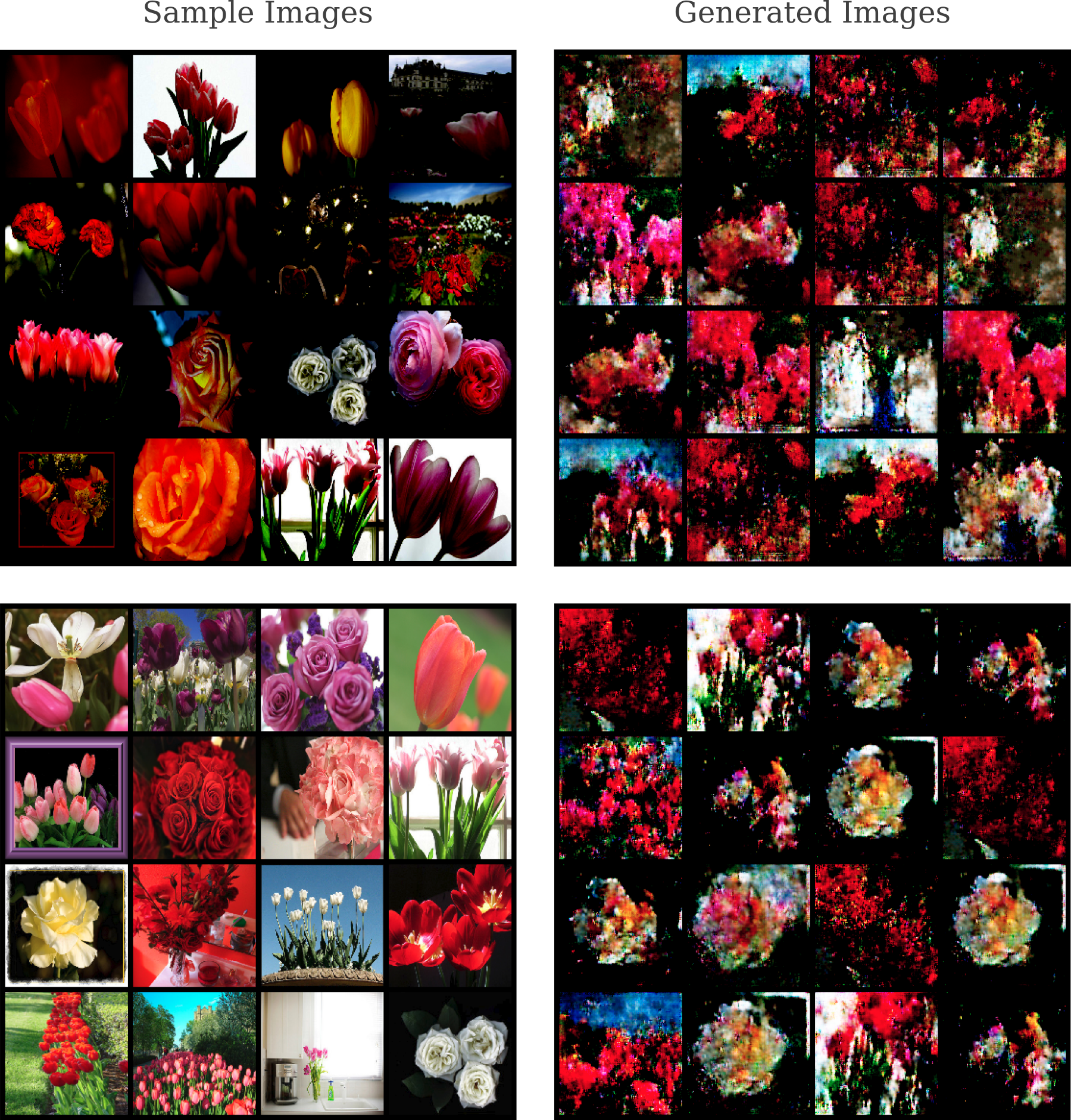
Spikes, ie sudden increases, are found uppon observing the generator’s loss function over time. This suggests that our architecture and design choices are not as stable as one would wish. Indeed, observing a subset of the generator’s outputs during learning shows that there are periods in which the model appears to ‘forget’ how to make accurate images of flowers and has to re-learn how to do so multiple times during the dataset. These correspond to times at which the discriminator is able to confidently reject all outputs by the generator, and appear in the following video when flower-like images dissipate into abstract patterns.

In the literature this is termed catastrophic forgetting, and is an area of current research in deep learning. Note that this phenomenon is also observed when an exact replica of the DCGAN architecture is used (with 64x64 input and generated image sizes, one less convolutional layer, no bias parameter in the fractional convolutional layers, and slightly different stride and padding parameters) and so is not the result of modifications made: instead it may be wondered if that the ‘forgetting’ is due to the very small sample size.

To test this idea, we can observe the stability of this architecture (modified slightly for 64x64 inputs) on a much larger dataset, say the 126,000 LSUN Churches dataset. Changing the resolution requires some small modifications to both generator and discriminator architectures if we use the DCGan approach, in this case making the resulting model more similar to the original one proposed by Radford and colleagues. This models is capable of rather quickly producing realistic-looking images of churches (albeit at low resolution) but it too suffers from instability during training: observe that at the end of the video below there is a lattice artefact introduced into each image and training progress ceases. This is because the discriminator’s loss for all images has zeroed out such that the generator no longer recieves a coherent error function.

Somewhat worryingly, the disappearance of the discriminator’s loss gradient is a regular occurrence for GANs of all types. The author has found this disappearance to be a common problem for everything from small, fully connected GANs applied to un-normalized MNIST monocolor datasets to larger cNN-based GANs applied to large datasets such as LSUN. This observation motivates the following question: why is the GAN objective function so unstable?

The first thing to note is that the reformulation of a zero-sum game introduced by Goodfellow and colleagues that has made GANs so effective and widespread was originally motivated by the observation that it prevented the disappearance of the generator’s loss gradient early in training, an outcome is typical of a zero-sum game implementation of a GAN. One may consider the derivation to be providing a Bayesian prior on the model specifying that input generation is more difficult than discrimination, which is why we make the loss function of the generator equivalent to the log-probability that the discriminator has made mistake rather than the loss function of the discriminator equivalent to the log-probability that the generator has not produced convincing samples.

However, once the generator begins to produce realistic samples then we may view the process of discrimination just as if not more difficult than generation. This motivates the use of both the Goodfellow reformulation as well as the alternative above…

Beyond this, however, we find other challenges to the GAN

More challenges of GANs

A fully connected architecture seemed to be effective for small (28x28) monocolor image generation using the MNIST datasets. Can a similar architecture applied to our small flower dataset yield realistic images? We can try a very large gut fairly shallow model: here the discriminator has the following architecture:

+------------------------+------------+
|        Modules         | Parameters |
+------------------------+------------+
| input_transform.weight | 100663296  |
|  input_transform.bias  |    8192    |
|       d1.weight        |  8388608   |
|        d1.bias         |    2048    |
|       d2.weight        |  1048576   |
|        d2.bias         |    512     |
|       d3.weight        |    512     |
|        d3.bias         |     1      |
+------------------------+------------+

and the generator mirrors this but with a latent space of 100, meaning that the entire network is over 230 million parameters which nears the GPU memory limit on colab for 32-digit float parameters.

This network and a half-sized version (half the first layer’s neurons) both make realistic images of flowers, but curiously explore a very small space: the following generator was trained using the same tulip and rose flower dataset as above, but only roses are represented among the outputs and even then only a small subset of possible roses (three to be specific) are generated.

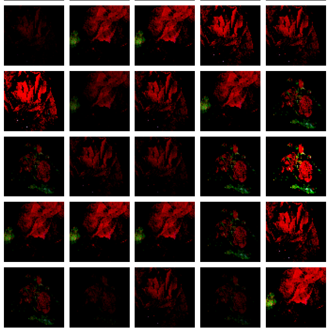
These images look quite realistic, but the truth is that they are far from what we want from a GAN: the are both overfit and underfit at the same time. Certain images in the dataset have been approximately copied, but the distribution over all flowers has clearly not been captured. This failure is known as ‘mode collapse’ which references the generator’s distribution over the inputs, $p_{model} (x)$, that assignes very high probability to only a few inputs $x$ (ie may modes $x_1, x_2, x_3,… x_n$ have collapsed into a few modes $x_1, x_2, x_3$ in the case above).

It is more common for GANs to exhibit a weaker version of mode collapse, in which more than a few but not all the distribution of inputs of the dataset, $x\sim p_{data}$, are represented. GANs typically develop sharp images that are visually realistic-looking (and can achieve low Frechet Inception Distance (FID) scores) but often ‘overlook’ certain inputs in doing so. This is not penalized by the typical measure of a generator network (best visual samples or FID score etc) but becomes a more serious issue for conditional image generation. Before exploring conditional generation, however, it is worth looking into how GANs may make higher-resolution images.

Increasing generator resolution

We have so far focused on the generation of low-resolution images, specifically those not exceeding 3x128x128. It is natural to wonder whether GANs may be used to generate higher-resolution inputs as well. Given that deep learning models applied to tasks of image classification often are effective accross a range of input resolutions, it may be assumed that the same is true of the DCGan architecture used in the last section.

Using the architectural choices of the DCGan for a higher-resolution image generation, we have the following generator (the discriminator mirrors this architecture) which takes a 1000-dimensional latent space vector and generates a color 512x512 output.

class StableGenerator(nn.Module):

	def __init__(self, minibatch_size):
		super(StableGenerator, self).__init__()
		self.input_transform = nn.ConvTranspose2d(1000, 2048, 4, 1, padding=0) # expects an input of shape 1x1000
		self.fc_transform = nn.Linear(100, 1024*4*4) # alternative as described in paper
		self.conv1 = nn.ConvTranspose2d(2048, 1024, 4, stride=2, padding=1) 
		self.conv2 = nn.ConvTranspose2d(1024, 512, 4, stride=2, padding=1)
		self.conv3 = nn.ConvTranspose2d(512, 256, 4, stride=2, padding=1)
		self.conv4 = nn.ConvTranspose2d(256, 128, 4, stride=2, padding=1)
		self.conv5 = nn.ConvTranspose2d(128, 64, 4, stride=2, padding=1)
		self.conv6 = nn.ConvTranspose2d(64, 32, 4, stride=2, padding=1)
		# switch second index to 3 for color images
		self.conv7 = nn.ConvTranspose2d(32, 3, 4, stride=2, padding=1) # end with shape minibatch_sizex3x512x512
		...

But when we apply this model to a dataset of 4k high-resolution images of landscapes, we find that the generator makes high-resolution but nonsensical images where a specific pattern or texture is repeated over and over.

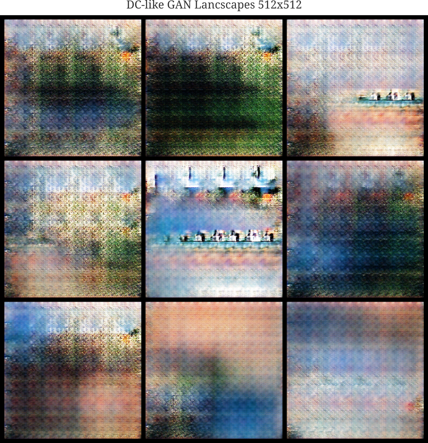
This problem has been observed in previous work, and is not too surprising when we consider all the ways that a generator could try to fool a discriminator. Instead of applying a large discriminator and generator pair to high-resolution images, we can instead use a stack of two models: first a low-resolution image is synthesizes by one generative adversarial network pair, and then this low-resolution map is converted to a high-resolution one with another GAN.

Directing GANs with latent space conditioning

Thus far we have been considering what is termred ‘unconditional’ image synthesis: given some dataset, the probability of a synthesized example $x_g$ of that dataset being similar to any one example $x_i$ is equal assuming that the GAN has not experienced mode collapse (which is unfortunately a rare scenario). It may be wondered how one can direct the synthesis system such that one type of input may be more likely to be generated