The genetic information problem
Background
Organisms can be viewed as the combination of the environment and heredity. In this work, we will consider mostly only heredity. The hereditery material of living organisms is (mostly) a polymer called deoxyribonucleic acid, usually referred to as DNA. The DNA forms very long strands in many cells, with some estimates putting the total length at over six feet per total DNA (called the genome) in each of ours.
A surprise came when the genomes of various animals and plants were first investigated: body complexity is not correlated with genome length. To give a particularly dramatic example of this phenomenon, it has been observed that the single-cell, half-millimeter-sized Amoeba proteus has a genome length of 290 billion (short billion, ie $10^9$) base pairs with is two orders of magnitude longer than our own (~3 billion base pairs).
When the human genome project was completed, the number of sections of DNA that encode proteins (genes) was estimated at around 22 thousand, which is not an inconsiderable number but far fewer than expected at the time. It was found that the vast majority of the human genome does not encode proteins but instead is a combination of repeat sequences left over from retroviruses, regulatory regions, and extended introns.
It could be hypothesized that the large amount of non-coding DNA is essential for the development of a complex body plan by providing extra regulatory regions. But even this is doubtful: the pufferfish Tetraodontidae rubripes contains a compact genome an eighth of the size of ours, and being a chordate retains an intricate body.
How then does the relatively small genome specify an incredibly detailed body of, for example, a vertebrate? In Edelman’s book Topobiology, a problem is laid out as follows: how can a one-dimensional molecule encode all the information necessary for a three-dimensional body plan for complicated organisms like mammals, given the incredible level of detail of the body plan?
Note that although the genome does have a three dimensional conformation that seems to be important to cell biology, any information stored in such shapes is lost between generations, that is, when egg and sperm nuclei fuse. This means that information contained in the complex three dimensional structure of the genome is lost, implying that it is the genetic code itself which provides most information.
An illustration: the memory of a 1D, 2D, and 3D arrays
To gain more perspective on what exactly the problem of storing information in a one dimensional chain like DNA, consider the memory requirements necessary to store 1- or 2- versus 3-dimensional arrays as a proxy for information content in each of these objects. We can do this using Python and Numpy.
# import third party libraries
import numpy as np
Now for our one dimensional array of size 10000 ($10^4$), populated with floating point numbers (64 bits each) with every entry set to 1, which represents our genome. Calling the method nbytes on this array yeilds its size,
x_array = np.ones((10000))
print (x_array.nbytes)
~~~~~~~~~~~~~~~~~~~~~~~~~~~~~~~~~~
80000
or 80 kilobytes. This is equivalent to about 5000 words, or the size of a chapter in a book. This is not a trivial amount of information, but now let’s look at the memory requirements of a two dimensional array of size ($(10^4)^2$) once again populated with floating point 1s:
xy_array = np.ones((10000,10000))
print (xy_array.nbytes)

~~~~~~~~~~~~~~~~~~~~~~~~~~~~~~~~~~
800000000
or 800 megabytes, around the size of the human genome. This makes sense, as if we square the 80 kilobytes we get 6.4 gigabytes, which is within an order of magnitude to what the program tells us about the memory here (the computed value being smaller means that the program stores the information cleverly to minimize its size).
Now lets try with a three dimensional array of size ($(10^4)^3$), representing our three dimensional body plan.
xyz_array = np.ones((10000, 10000, 10000))
print (xyz_array.nbytes)
Our program throws an exception
~~~~~~~~~~~~~~~~~~~~~~~~~~~~~~~~~~
Traceback (most recent call last):
...
MemoryError: Unable to allocate 7.28 TiB for an array with shape (10000, 10000, 10000) and data type float64
[Finished in 0.2s with exit code 1]
but at have our answer: the three dimensional array is a whopping 7.28 terabytes. This is a thousand times the size of the memory of most personal computers so it is little wonder that we get an error!
The increase from 80 kilobytes to 7.28 terabytes demonstrates that there is far more informational content in a three dimensional object than in an object of one.
Now let’s look at scaling in order to see by how much dimensional genome should increase in length when an organism increases in complexity. Say that we are working with a coral, Acropora millepora that has a genome of around 400 million base pairs. Here is a picture of an acropora (not millepora sp.) from my aquarium:
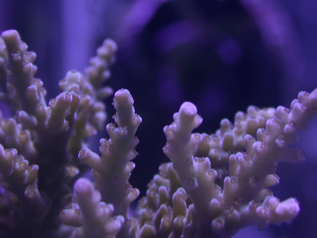
Like all cnidarians, this coral has a simple blind-ended digestive system, a small web of neurons, and little mesoderm. It is a colonial polyp, meaning that each of the small rings you see are an individual animal that is fused to the rest of the coral. Now imagine that its body were over the course of evolution to acquire more adaptive features like ten times as many neural-like cells and ten times the number of cnidocytes, the cells that have tiny harpoon-like stingers that trap prey and deter preditors. As an approximation, say that the three dimensional plan becomes ten times as information intensive. How much would the one dimensional strand of DNA have to increase to accomodate this new information? $ 10 ^ 3 = 1000$, in other words we would expect a new genome size of around 400 billion base pairs. This is three times the size of the largest genome currently found for any animal (Protopterus aethiopicus, the lungfish), and is over a hundred times the size of our genome!
But as recounted in the introduction with dramatic examples, there is little correlation between genome size and body complexity. This means that there is no scaling at all, but how is this possible?
To sum up the problem in a sentence: the human genome is ~750 megabytes (2 bits per nucelotide, 3 billion nucleotides, and 8 bits per byte yields 750 million bytes), which is less information than is contained in one three dimensional reconstruction of a single neuron with an electron microscope.
What genomes specify
How can such a small amount of information encode something so complex? The simple answer is that it cannot, at least not in the way encoding is usually meant.
Consider the other pages of this website. There, we see many examples of small and relatively simple equations give rise to extremly intricate and infinitely detailed patterns. An important thing to remember about these systems are that they are dynamical: they specify a change over time, and that they are all nonlinear (piecewise linear equations can also form comlicated patterns, but for our purposes we can classify piecewise linear equations as nonlinear).
If simple nonlinear dynamical equations can give rise to complex maps, perhaps a relatively simple genetic code could specify a complex body by acting as instructions not for the body directly but instead for parameters that over time specify a body. In this way, the genetic code could be described as a specification for a nonlinear dynamical system of equations rather than a simple blueprint that can be read.
Why does this help the genome specify a detailed three dimensional body from a single dimension? Suppose we wanted to store the information necessary to create a complex structure like a zoomed video of a Julia set. The ones I made were usually around 80 megabytes for 10 seconds worth of video. It would take 100 seconds to make a movie that is 800 megabytes in size (without compression), just larger than the human genome. And this is only for one among a multitute of possible locations to increase scale and still recieve more information! A very detailed version of a Julia set would take a prodigous amount of memory to store, wouldn’t it?
No, because the dynamical equation specifying the specific Julia set gives us all the information we need. This is because dynamical systems are deterministic: one input yields one output, no chance involved. All we need is to store this equation
\[z_{next} = z_{current}^2 + a\]and then have a system that computes each iteration. In text, this is only 25 bytes, but gives us the incredibly information-rich maps of the set. In this sense, an extremely complicated structure may be stored in with a miniscule amount of information.
Iterated Information
Considering the transmission of binary electrical signal over a noisy background, Shannon defined binary informational entropy as follows:
\[H = -\left( p \log_2(p) + q \log_2(q) \right)\]where $p$ is the probability of transmitting a certain signal (perhaps ‘1’) and $q = 1-p$, or the probability of not recieving the other signal, and $H$ is the information entropy in bits (binary digits) per signal. ‘Entropy’ here has little to nothing to do with the entropy of physical substances, but rather is a measure of total informational amount: the more entropy a transmission contains, the more information it transfers. Plotting this equation with $H$ on the y-axis and $p$ on the x-axis,
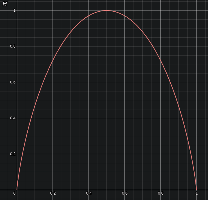
Informational entropy is maximized when $p = q = 0.5$, which at first may seem strange. After all, a simple random distribution of 0s and 1s, or heads and tails if one wished to flip coins, would also yield $p = q = 0.5$. Why does approaching a random distribution give more information?
One way to see this is to consider what would happen if $p = 1, q = 0$: now every signal received is a $1$, and so there is minimal new information (as we could already predict that the signal would be $1$ at any given time). On the other hand, a signal consisting more unpredictable sequence of 1s and 0s intuitively yields more informational content. A completely unpredictable distribution of 1s and 0s would be (without prior knowledge) indistinguisheable from noise.
Say one were attempting to communicate with a friend by sending messages back and forth over an unconventional transmission line. This transmission line changes such that each time a message is sent, the probability of a $1$ being recieved at any position of the message is equal to the entropy (in bits) of the message recieved. Tracking the entropy of each message over time can be accomlished using the dynamical system:
\[x_{n+1} = - \left( x_n \log_2 (x_n) + (1-x_n) \log_2 (1-x_n) \right)\]which when starting near $x_0 = 0.299$ gives the following graph:
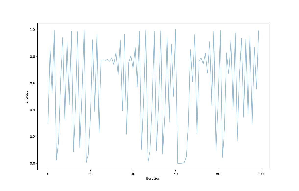
which itself looks like noise! The entropy moves around unpredictably, not settling on any value over time.
Now real electrical transfer is usually lossy, meaning that whatever sequence of 0s and 1s we send will likely not arrive so cleanly, but instead as for example $0,1,0,1,1…$ may become $0.12, \; 0.99,\; 0.01,\; 0.87,\; 0.62…$. In this case we are not exactly sure what the signal was intended to be, meaning that some information is lost.
Repeating the same process of tracking entropy over time as messages are sent and received, we have
\[x_{n+1} = - a\left( x_n \log_2 (x_n) + (1-x_n) \log_2 (1-x_n) \right)\]where $a$ is defined as a constant of loss: $a=1$ signifies no signal loss, $a=0$ means all sigal is lost. Making an orbit map at different values of $a$,
#! python3
# Import third-party libraries
import numpy as np
import matplotlib.pyplot as plt

def information_map(x, a):
	return - a * (x*np.log2(x) + (1-x)*np.log2(1-x))

a_ls = [0.5]
x_ls = [0.1]

steps = 1000000

for i in range(steps):
	a_ls.append(a_ls[-1] + 0.5/steps)
	x_ls.append(information_map(x_ls[-1], a_ls[-1]))

plt.plot(a_ls, x_ls, ',', color='black', alpha=0.1, markersize=0.1)
plt.axis('on')
plt.xlabel('Loss factor')
plt.ylabel('Informational entropy')
there is
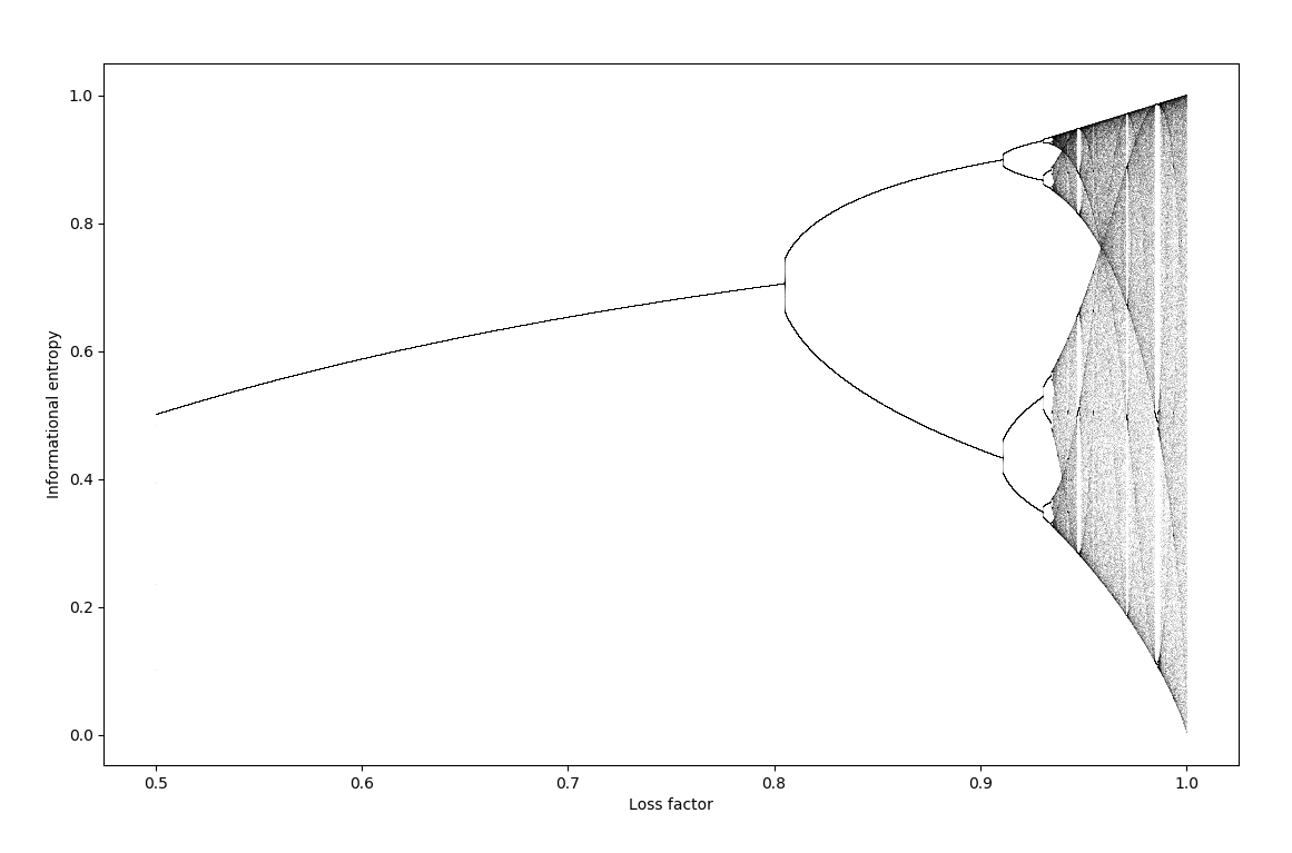
This is a period-doubling behavior analagous to the logistic map.
Instructional information
How can we reconcile the observations above of very low-information instructions leading to complicated, even unpredictable outputs that by Shannon’s definition have a very large informational content?
Much of computer science can be thought of as belonging either to the study of information transfer, or the study of computation. Shannon’s definition of information is based on communication from a source to a reciever, which is clearly applicable to the real world with respect to transfer of information. But our observations above are of a computational nature, and this motivates a different definition of information (but one that closely corresponds with Shannon’s).
Definition: instructional (computational) information amount is the number of steps specified before the procedure repeats itself endlessly or halts.
This is most clearly understood in the context of the theory of general recursive functions, which we can substitute with Turing machines. First note that a limited number of Turing machine input specifications can yield a very large number of possible instructions (before looping or halting). A further discussion of steps taken given a Turing machine input may be found elsewhere. But for the sake of illustration, the maximum number of steps possible given a Turing machine with two symbols and n possible states, denoted $s(2, n)$ is (as documented here):
\[s(2, 2) = 6 \\ s(2, 3) = 21 \\ s(2, 4) = 107 \\ s(2, 5) = 47,176,870 \\ s(2, 6) > 7.4 × 10^{36534}\]This number grows at an incredible rate: its precise growth is uncomputable due to the fact that the halting problem itself is undecidable.
This definition of information is similar to Shannon’s with respect to the amount of information, termed informational entropy in Shannon’s parlance. For instructional information, a truly random input would have an infinite number of instructions without ever halting or looping and this mirrors how the maximum Shannon informational entropy is achieved for a random-like input. This is an important quality to retain, as it is clear that storage of real data that is noisy, or stochastic, is much more information-heavy than storage of non-noisy data.
Using the number of instructions as a definition for informational content, we can clearly see that a function with very few inputs can result in an extremely large informational output, which was what we wanted.
The process of protein folding
To the eye of someone used to thinking of the genome as a collection of genes that are ‘read’ during protein transcription, the idea that the genome does not directly encode information yielding a three dimensional product may be counterintuitive. After all, this seems to be how proteins are made: the genetic code is read out almost like a tape by RNA polymerase, which then is read out (again sequentially) by the ribosome. The three-nucleotide genetic code for each amino acid has been deciphered and seems to point us to the idea that the genome is indeed a source of information that is stored as blueprints, or as a direct encoding. Is there any evidence for the idea that information in genetic are stored as instead instructions for nonlinear dynamical systems?
Let us consider the example of proteins (strings of amino acids) being encoded by genes more closely. Ignoring alternative splicing events, the output of one gene is one strand of mRNA, and this yields one strand of amino acids. But now remember that the strand of amino acids must fold to make a protein, and by doing so it changes from one dimension to three. It is in this step that we can see the usual traits of nonlinear dynamical systems come in to play, and these features deserve enumeration.
First, protein folding is a many-step process and is slow on molecular timescales. This means that there is an element of time that cannot be ignored. As dynamical systems are those that change over time, we can define protein folding as a dynamical system. Protein folding usually proceeds such that nonpolar amino acids collect in an interior whereas polar and charged amino acids end up on the exterior, and this takes between microseconds to seconds depending on the protein ref, far longer than the picosecond time scales in which molecular bond angles change.
This is not surpising, given that a protein with a modest number of 100 amino acids has $3^{100}$ most likely configurations (3 chemically probable orientations for 100 side chains) ref. But viewing a Ramachandran plot of bond angles of peptides is sufficient to show us that these three orientations are not all-encompassing, nor discrete: there are far more actual bond configurations than three per amino acid. This means that a more accurate number of orientations for our 100 amino acids is far larger than $3^{100}$.
It is apparent that proteins do not visit each and every configuration while folding, for if they did then folding would take $10^{27}$ years, an observation known as Levinthal’s paradox. It is clear that a folding protein does not visit every possible orientation, but instead only a subset of these before settling on a folded state. The orientations that are visited are influenced by every amino acid: the folding is in this way nonlinear as it is not additive, meaning that the effects on the final protein of a change in one amino acid cannot be determined independantly of the other amino acids present. As it is dynamical, protein folding may be described as aperiodic, ie non-repeating, unless the folded protein is exactly the same as the unfolded amino acid chain.
Second, protein folding is sensitive to initial conditions. A chemically significant (nonpolar to ionic, for example) change in amino acid quality may be enough to drastically change the protein’s final shape, an example of which is the E6V (charged glutamic acid to nonpolar valine) mutation of Hemoglobin.
But note that this sensitivity does not seem to extend to the initial bond angles for a given amino acid chain, only to the amino acids found in the chain itself (otherwise thermal motion to identical chains would be expected to yield different folded conformations). In this way protein folding resembles the formation of a strange attractor like the Clifford attractor where many starting points yield one final outcome, but these starting points are bounded by others that result in a far different outcome.
Finally, protein folding is difficult to predict: given a sequence of DNA, one can be fairly certain as to what mRNA and thus what amino acid chain will be produced (ignoring splicing) if that sequence of DNA has never been seen before. But a similar task for predicting a protein’s folded structure based on its amino acid chain starting point has proven extremely challenging for all but the smallest amino acid sequences.
The reason for this is often attributed to the vast number of possible orientations an amino acid may exist in, but it is important to note that there are a vast number of possible sequences of DNA for each gene (if there are 100 nucleotides, there are $4^{100}$ possibilities) but that we can predict the amino acid sequences from all these outcomes regardless. If we instead view this problem from the lense of nonlinear dynamics, a different explanation comes about: sensitivity to initial conditions implies aperiodicity, and aperiodic dynamical systems are intrinsically difficult to predict in the long term.
Implications for cellular and organismal biology
We have seen how protein folding displays traits of change over time, aperiodicity, sensitivity to initial conditions and difficulties in long-term prediction. These are traits of nonlinear dynamical systems, and the latter three are features of chaotic dynamical systems. What about at a larger scale: can we see any features one would expect to find in a nonlinear dynamical system at the scale of the tissue or organism?
Self-similarity is a common feature of nonlinear dynamical systems, and for our purposes we can define this as object where a small part of the shape resembles the whole. This can be exactly geometric similarity as observed in many images of dynamical boundaries or else approximate (also known as statistical) self-similarity, where some qualitative aspect of a portion of an object resembles some qualitative aspect of the whole, which manifests itself as a fractal dimension. For a good introduction to fractals see here, and note that in this context a fractal dimension is an indicator of approximate self-similarity and that the phrase ‘self-similarity’ in this video is limited to perfect geometrical self-similarity.
Most tissues in the human body contain some degree of self-simimilarity. This can be most clearly seen in the branching patterns of bronchi in lungs and the arteries, arterioles, and capillaries of the circulatory system. But in many organs, the shapes of cells themselves often reflects the shape of the tissue in which they live, which reflects the organ. For instance, neurons are branched and elongated cells that inhabit a nervous system that is itself branched and elongated at a much larger scale.
Temporal self-similarities in living things and and the implications of nonlinear dynamics in homeostasis and development are considered elsewhere.
Reproduction and information
On other pages of this site, self-similar fractals resulting from simple instructions are found. Many such maps contain smaller versions of themselves ad infinitum, meaning that one can see at any arbitrary scale the whole figure. Except in cases of trivial self-similarity (like that existing for a line), such objects are of infinite information. THe images of fractals on this and other sites are only finite representations of the true figures.
Self-similar fractals may seem far removed from biology, but consider the ability of living organisms to reproduce. With the acceptance of cell theory in the 1800s (the idea that multicellular organisms such as humans are composed of many smaller organisms) brought about a difficulty for understanding reproduction. How can the information necessary to make an entire person reside in a single cell? One theory (predating acceptance of cell theory) was the existance of a homonculus, a small person resided in a gamete. But in this small person must exist another gamete containing an even smaller person and so on.
The homunculus was discarded after closer examination revealed no such person inside gamete cells. But reproduction does bring a difficult question with regards to information. Consider the simpler case of an asexually reproducing single cell: the genetic information contained inside one individual is also enough information for other individuals as well. The apprently limitless capacity for reproduction (as long as enviromental conditions are optimal) means that a finite amount of information contained in the genetic material of one cell has the potential to specify any arbitrary number of cells. This applies even when the original cell only divides a certain number of times before scenescence (as for budding yeast, for example) because as long as each cell divides once, exponential growth occurs.