Gradients are sensitive to minibatch composition

This idea runs somewhat against the current grain of intuition by many researchers, so reading the preceding paragraphs was probably not sufficient to convince an active member in the deep learning field. But happily the concept may be shown experimentally and with clarity. Take a relatively small network being trained to approximate some defined (and non-stochastic) function. This practically any non-trivial function, and here we will focus on the example detailed on this page. In this particular case, a network is trained to regress an output to approximate the function

\[y = 10d\]

where $y$ is the output and $d$ is one of 9 inputs. The task is simple: the model must learn that $d$ is what determines the output, and must also learn to decipher the numerical input of $d$, or in other words the network needs to learn how to read numbers that are given in character form. A modest network of 3.5 million parameters across 3 hidden layers is capable of performing this task extremely accurately.

In the last section, the landscape of $h$ was considered. Here we will focus on the gradient of $h$, as stochastic gradient descent is not affected by the values of $h$ but only their rate of change as $\theta$ chages. We can observe the gradient of the objective function $J(O(a; \theta))$ with respect to certain trainable parameters, say two parameters in vector form $x = (x_1, x_2)$. The gradient is signified by $\nabla_x J(O(a; \theta))$ and resulting vector is two dimensional and may be plotted in the plane, as $x$ is equivalent to the projection of the gradient $\nabla_\theta J(O(a; \theta))$ onto our two parameters. But we are interested in more than just the gradient of the parameters: we also want to visualize the landscape of the possible gradients nearby, that is, the gradients of $\nabla_x J(O(a; \theta), y)$ if we were to change the parameter $x$ slightly, as this is how learning takes place during SGD. The gradient landscape may be plotted by assigning gradients to points on a 2-dimensional grid of possible values for the parameters $(x_1 + \epsilon_n, x_2 + \epsilon_n)\; n \in \Bbb Z$ that are near the model’s true parameters $x$. In the following plot, the $\nabla_x J(O(a; \theta), y)$ vector is located at the center circle, and the surrounding vectors are the gradients $\nabla_{x’} J(O(a; \theta), y)$ with $x’$ signifying $x_1+\epsilon_n, x_2 + \epsilon_n$

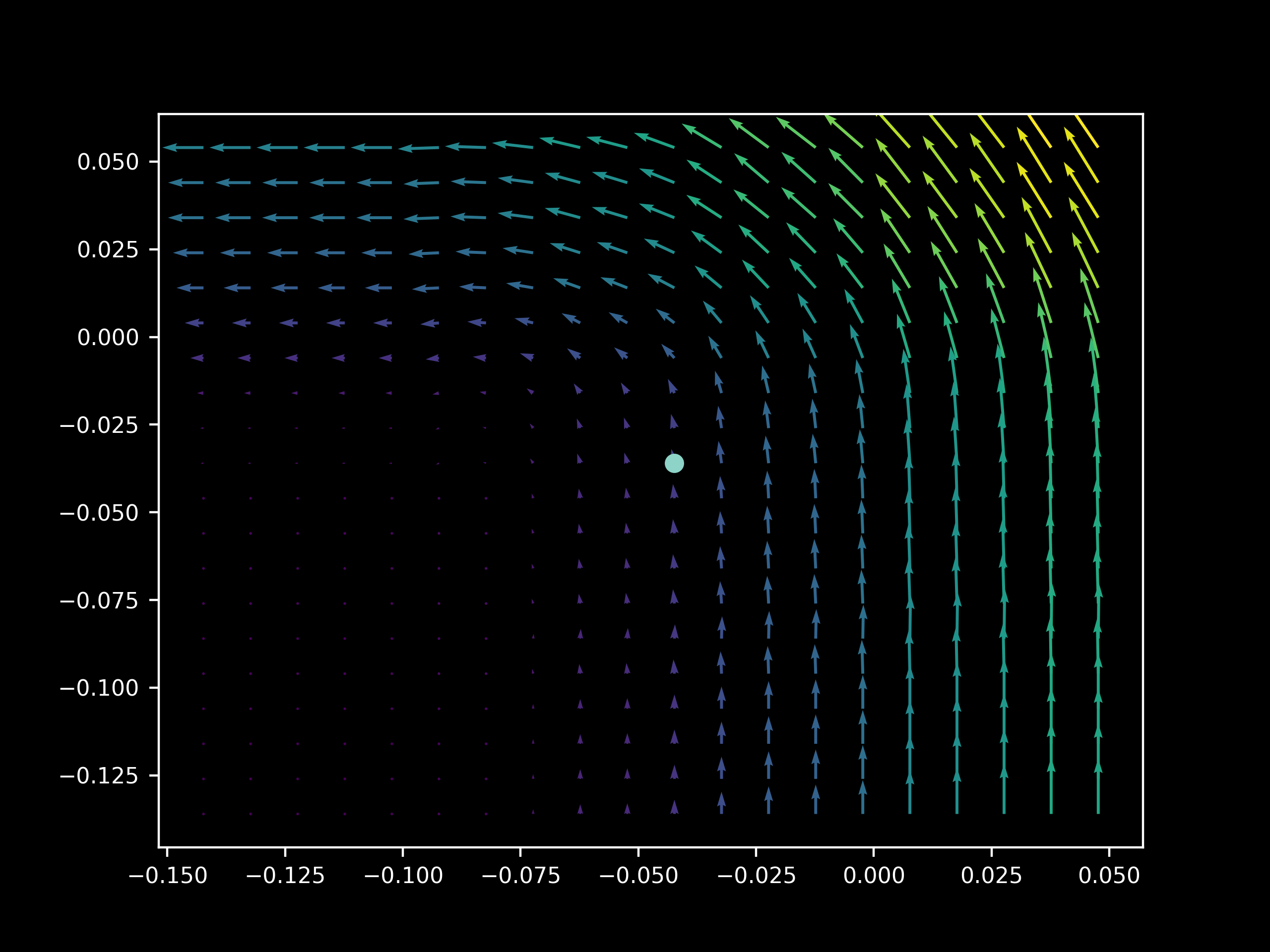
Because our model is learning to approximate a deterministic function applied to each input, the classical view of stochastic gradient descent suggests that different subsets of our input set will give approximately the same gradient vectors for any given parameters, as the information content in each example is identical (the same rule is being applied to generate an output). In contrast, our idea is that we should see significant differences in the gradient vectors depending on the exact composition of our inputs, regardless of whether or not their informational content is identical w.r.t. the loss function.

Choosing an epoch that exhibits a decrease in the cost function $J(O(a; \theta), y)$ (corresponding to 6 seconds into this video) allows us to investigate the sensitivity (or lack thereof) of the model’s gradients to input $a$ during the learning process. As above the gradient’s projection onto $(x_1, x_2)$ is plotted but now we observe the first two bias parameters in two hidden layers. The model used on this page has three hidden layers, indexed from 0, and we will observe the gradient vectors on the second and third layer.

One can readily see that for 50 different minibatches $a_1, a_2,…,a_{50} \in a$ (each of size 64) of the same training set, there are quite different (sometimes opposite) vectors of $\nabla_x J(O(a_n; \theta), y)$

In contrast, at the start of training the vectors of $\nabla_x J(O(a; \theta), y)$ tend to yield gradients on $x$ that are (somewhat weak) approximations of each other.

Regularization is the process of reducing the test error without necessarily reducing training error, and is thus important for overfitting. One nearly ubiquitous regularization strategy is dropout, which is where individual neurons are stochastically de-activated during training in order to force the model to learn a family of closely related functions rather than only one. It might be assumed that dropout prevents this difference in $\nabla_x J(O(a; \theta), y)$ between minibatches during training, but it does not: we still have very different gradient landscapes depending on the input minibatch. Note too how dropout leads to unstable gradient landscapes, where adjacent gradient projections are unpredictably different from one another.

but once again this behavior is not as apparent at the start of training

Another technique used for regularization is batch normalization. This method is motivated by an intrinsic problem associated with deep learning: the process of finding the gradient of the cost function $J$ with respect to parameters $x$ with respect to the cost function $\nabla_x J(O(a; \theta), y)$ may be achieved using backpropegation, but the gradient descent update of $x$, specifically $x - \epsilon\nabla_x J(O(a; \theta), y)$, assumes that no other parameters have been changed. In a one-layer (inputs are connected directly to outputs) network this is not much of a problem because the contribution of $x_n$ (ie the weights) to the output’s activations are additive. This is due to how most deep learning models are set up: in a typical case of a fully connected layer $h$ following layer $h_{-1}$ given the weight vector for that neuron $w$ and bias scalar $b$

\[h = w^Th_{-1} + b\]

where $w^Th_{-1}$ is a vector dot product, a linear transformation that adds all $w_nh_{-1,n}$ elements. The gradient is computed and updated in (linear) vector space, so if a small enough $\epsilon$ is used then gradient descent should decrease $J$, assuming that computational round-off is not an issue.

But with more layers, the changes to network components becomes exponential with respect to the activations at $h$. To see why this is, note that for a four-layer network with biases set to 0 and weight vectors all equal to $w$

\[h = w^T(w^T(w^T(w^Th_{-4})))\]

Now updates to these weight vectors, $w - \epsilon\nabla_w J(O(a; \theta), y)$ are no longer linear with respect to the activation $h$. In other words, depending on the values of the components of the model a small increase in one layer may lead to a large change in other layers’ activations, which goes against the assumption of linearity implicit in the gradient calculation and update procedure.

Batch normalization attemps to deal with this problem by re-parametrizing each layer to have activations $h’$ such that they have a defined standard deviation of 1 and a mean of 0, which is accomplished by using the layer’s activation mean $\mu$ and standard deviation $\sigma$ values that are calculated per minibatch during training. The idea is that if the weights of each layer form distributions of unit variance around a mean of 0, the effect of exponential growth in activations (and also gradients) is minimized.

But curiously, batch normalization also stipulates that back-propegation proceed through these values $\sigma, \mu$ such that they are effectively changed during training in addition to changing the model parameter. Precisely, this is done by learning new parameters $\gamma, \beta$ that transform a layer’s re-paremetrized activations $h’$ defined by the function

\[h'' = \gamma h' + \beta\]

which means that the mean is multiplied by $\gamma$ before being added by $\beta$, and the standard deviation is multiplied by $\gamma$. This procedure is necessary to increase the ability of batch normalized models to approximate a wide enough array of functions, but it in some sense defeats the intended purpose of ameliorating the exponential effect, as the transformed layer $h’’$ has a mean and standard deviation can drift from the origin and unit value substantially. Why then is batch normalization an effective regularizer?

Let’s investigate by applying batch normalization to our model and observing the effect on the gradint landscape during training. When 1-dimensional batch normalization is applied to each hidden layer of our model above, we find at 10 epochs that $\nabla_x J(O(\theta; a), y)$ exhibits relatively unstable gradient vectors in the middle layer. As we saw for dropout and non-regularized gradients, different minibatches have very different gradient landscapes.

Thus we come to the interesting observation that batch normalization leads to a similar loss of stability in the gradient landscape that is seen for dropout. which in this author’s opinion is a probable reason for its success as a regularizer (given dropout’s demonstrated success in this area). This helps explain why it was found that batch normalization and dropout are often able to substitute for each other in large models: it turns out that they have similar effects on the gradient landscape of hidden layers, although batch normalization in this case seems to be a more moderate inducement of this loss of stability.

Note that for each of the above plots, the model’s parameters $\theta$ did not change between evaluation of different minibatches $a_n$, of in symbols there is an invariant between $\nabla_x J(O(a_n; \theta), y) \; \forall n$. This means that the direction of stochastic gradient descent does indeed depend on the exact composition of the minibatch $a_n$.

To summarize, we find that the gradient with respect to four parameters can change drastically depending on the training examples that make of the given minibatch $a_n$. As the network parameters are updated between minibatches, both the identity of the inputs per minibatch and the order in which the same inputs are used to update a network determine the path of stochastic gradient descent. This is why the identity of the input $a$ is so important, even for a fixed dataset with no randomness.