Logistic Map

Introduction: periodic trajectories in the logistic map

The logistic map was derived from a differential equation describing population growth, popularized by Robert May. The dynamical equation is as follows:

\[x_{n+1} = rx_n (1 - x_n) \tag{1} \label{eq1}\]

where r can be considered akin to a growth rate, $x_{n+1}$ is the population next year, and $x_n$ is the current population. Population ranges between 0 and 1, and signifies the proportion of the maximum population.

Let’s see what happens to population over time at a fixed r value. To model \eqref{eq1}, we will employ numpy and matplotlib, two indispensable python libraries.

#! python3
# import third-party libraries
from matplotlib import pyplot as plt 
import numpy as np 

# initialize an array of 0s and specify starting values and r constant
steps = 50
x = np.zeros(steps + 1)
y = np.zeros(steps + 1)
x[0], y[0] = 0, 0.4

r = 0.5

# loop over the steps and replace array values with calculations
for i in range(steps):
	y[i+1] = r * y[i] * (1 - y[i])
	x[i+1] = x[i] + 1

# plot the figure!
fig, ax = plt.subplots()
ax.plot(x, y, alpha=0.5)
ax.set(xlabel='Time (years)', ylabel='Population (fraction of max)')
plt.show()

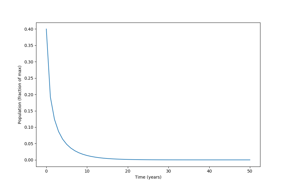
When $r$ is small (less than one, to be specific), the population heads towards 0. Here $r=0.5$:

As $r$ is increased to 2.5, a stable population is reached:

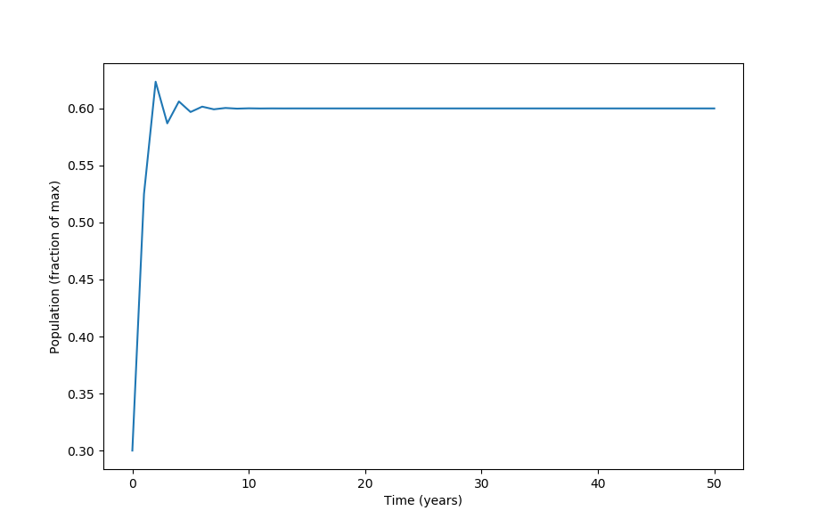
This is called a period one trajectory because it takes one iteration to return to the starting population size. Because period one occurs when $x_{n+1} = x_n$, we can algebraically determine the population values reached. At $r=2.5$ we have

\[x_n = 2.5x_n(1-x_n) \\ 0 = -2.5x_n^2 + 1.5x_n = x_n \left( -\frac{5}{2}x_n+\frac{3}{2} \right) \\ x_n = 0, \; x_n = 3/5 \\\]

where the value of $x_n = 3/5$ is an attractor for all initial values except for 0, and $x_{n+1} = 0$ only occurs for $x_0 = 0$. An attractor in a dynamical system such as this is a point that other points head towards, and in this $x_n = 3/5$ is an attractor for all starting points $x_0 \in (0, 1)$.

How can one tell that $x_n = 3/5$ is an attractor but $x_n = 0$ is not? One way is simply to start from a number of different points and see where future iterations end up: this was used above. But this method can be difficult and imprecise when many values are to be tested, so it is often best to try to determine whether or not a point is an attractor by using the following analytical method.

Stability for one-dimensional systems may be determined using linearization, and for iterated equations like the logistic map this involves determining whether or not the absolute value slope of the derivative of $f(x)$ is less than one, or $\lvert f’(x) \rvert < 1$. If so, the point is stable but if $\lvert f’(x) \rvert > 1$, it is unstable (and if it equals one, we cannot say). For the logistic equation, $f’(x) = r-2rx$ and so at $r=2.5$,

\[f'(x) = r - 2rx_n \\ f'(x) = 3.5-7x_n \\ f'(0) = 3.5-0 > 1\]

and therefore $x=0$ is unstable. On the other hand, $f’(3/5) = 3.5-4.2 = -0.7$ which means that $x=3/5$ is a stable point of period 1. As we shall see below, stable points of finite period act as attractors, such that points in $(0, 1)$ eventually end up on the point $x=3/5$ given sufficient iterations.

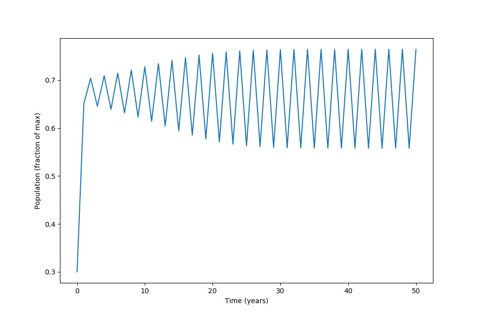
Returning to models of \eqref{eq1{, at $r = 3.1$ the population fluctuates, returning to the starting point every other year instead of every year. This is called ‘period 2’:

At this r value, can find points where $x_{n+1} = x_n$ (meaning points of period one),

\[x_n = rx_n(1-x_n) \\ 0 = x_n(2.1-3.1x_n) \\ x_n = 0, x_n \approx 0.677\]

but some quick numerical experimentation shows that these points are unstable: any slight deviation from the values (and indeed any finite approximation of 0.677…) will not result in $x_{n+1} = x_n$.

Points of period 2 may be found as follows:

\[f(f(x)) = f^2(x) = x \\ x = r^2x(1-x)(1-rx(1-x)) \\ 0 = x(-r^3x^3 + 2r^3x^2 - (r^3+r^2)x + r^2 - 1)\]

which when $r=3.1$ has a root at $x=0$. The other roots may be found using the rather complicated cubic equation, and are $x\approx 0.76457, x \approx 0.55801, x \approx 0.67742$. Note that the two unstable period-1 points are included (see below), but that there are two new points. To see if they are stable, we can check if $\lvert (f^2)’ \rvert < 1$, and indeed as $(f^2)’(x) = -4r^3x^3 + 6r^3x^2 - 2\left(r^3+r^2\right)x + r^2$, and substituting both $x=0.55801$ and $x=0.76457$ yields a number around $\lvert 0.5899.. \rvert < 1$, meaning that both points are stable. Therefore both are attractors, as seen in the previous numerical map. On the other hand, $(f^2)’(0.67742) = 1.21$ and $(f^2)’(0) = 9.61$, neither of which are between positive and negative one and thus both points are unstable. The point $x\approx 0.67742$ would be stable if the period had not increased: this is a period-doubling bifurcation.

Note that ‘period’ on this page signifies what is elsewhere sometimes referred to as ‘prime period’, or minimal period. Take a fixed point, for example at $r=2.5$ this was found to be located $x=3/5$. This has period 1 because $x_{n+1} = x_n$, but it can also be thought to have period 2 because $x_{n+2} = x_n$ and period 3, and any other finite period because $x_{n+k} = x_n \forall k$. This is why we found period-1 points when trying to compute period-2 values above.

But there is a clear difference between this sort of behavior and that where $x_{n+2} = x_n$ but $x_{n+1} \neq x_n$, where the next iteration does not equal the current but two iterations in the future does. The last sentence is true for the logistic map where $r=3.1$, and we can call this ‘prime period 2’ to avoid ambiguity. But for this and other pages on this site, ‘prime’ is avoided as any specific value referred to by ‘period’ is taken to mean ‘prime period’.

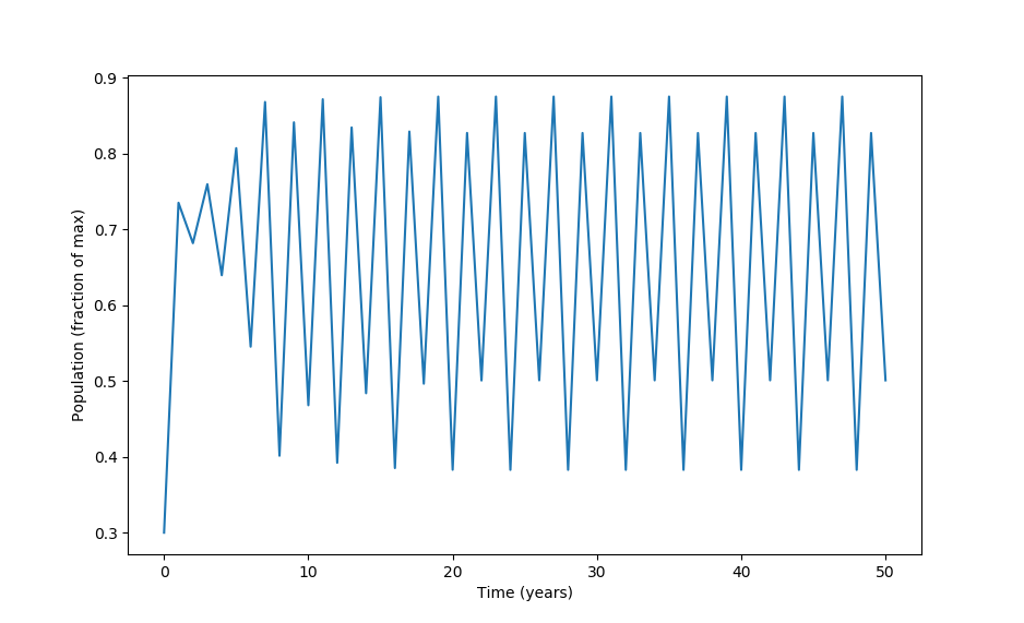
at $r = 3.5$, the trajectory is period 4, as it takes 4 iterations for the population to return to its original position:

As $r$ increases, trajectories of $8,\; 16,\; 32,\; 64…$ exist: given any natural number that is the power of two, there is some $r$ value range for which the logistic map trajectory has that number as a periodic cycle.

Aperiodic trajectories in the logistic map

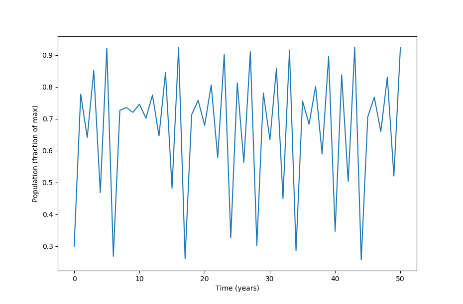
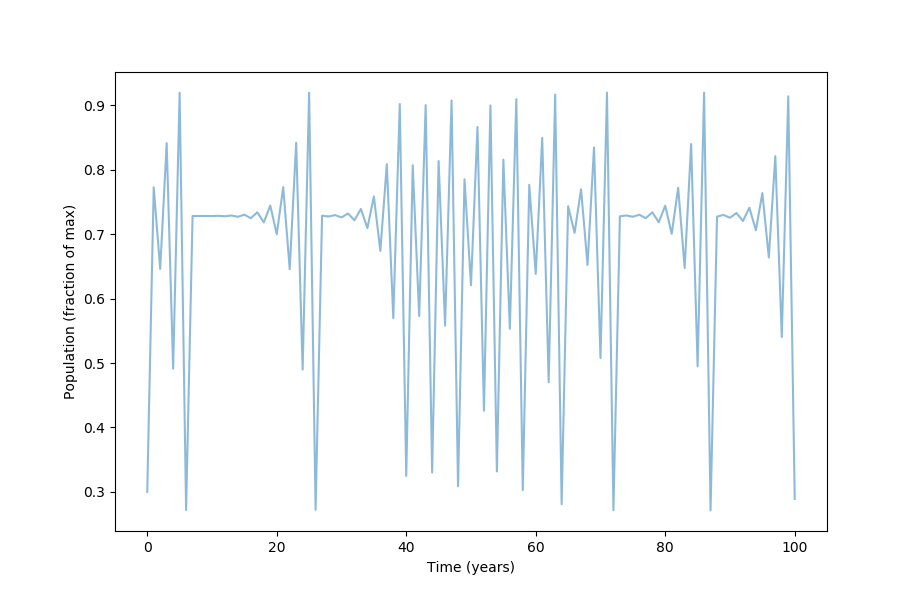
For $r=3.7$, the (prime) period is longer than the iterations plotted and is actually infinite, and therefore the system is called aperiodic. To restate, this means that previous values of the logistic equation are never revisited for an aperiodic $r$ value. The ensuing plot has points that look random but are deterministic. The formation of aperiodic behavior from a deterministic system is termed mathematical chaos.

Are there any non-prime periodic points? Looking for points of period 1 (keeping $r=3.7$), we find two:

\[x_n = rx_n(1-x_n) \\ 0 = x_n(2.7-3.7x_n) \\ x_n = 0, \; x_n = 27/37\]

Both are unstable, as $f’(0) = 3.7 - 2 \cdot 3.7 \cdot 0 > 1$ and $f’(27/37) = 3.7 - 54/37 > 1$. For points of period 2, the cubic formula can be used to find

\[0 = x_n(-r^3x_n^3 + 2r^3x_n^2 - (r^3+r^2)x + r^2-1) \\ x_n = 0, \; x_n = 27/37 \; x_n \approx 0.88, \; x_n = 0.39\]

the fixed points are found again, and in addition two more points are found. All are unstable (which can be checked by observing that all points fail the test of $\lvert (f^2)’(x_n) \rvert < 1$). What makes the $r=3.7$ value special is that for any given integer $k$, one can find periodic points with period $k$. But as $k+1$ also exhibits periodic points, the logistic map with $r=3.7$ only has a prime periodic point at $x_n = \infty$, which is to say that the map has no finite (prime) periodic points and therefore aperiodic.

As demonstrated by Lorenz in his pioneering work on flow, nonlinear dissipative systems capable of aperiodic behavior are extremely sensitive to initial conditions such that long-range behavior is impossible to predict.

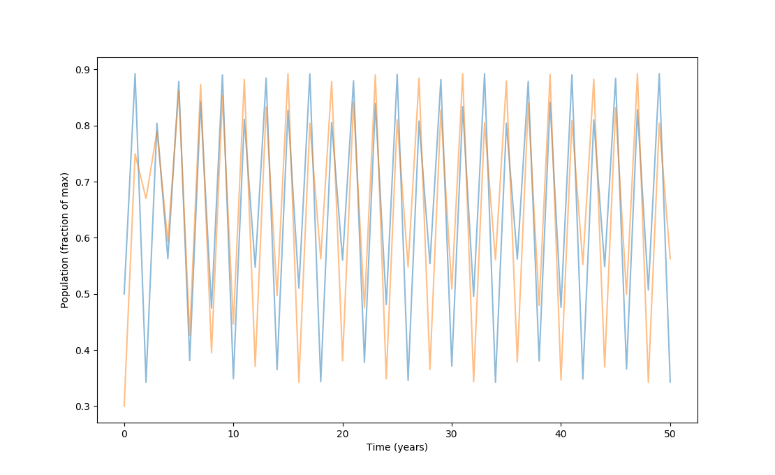
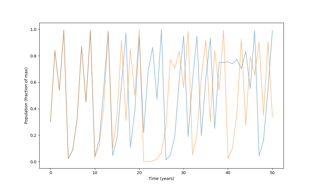
Observe what happens when the starting population proportion is shifted by a factor of one ten-millionth with $r=3.7$:

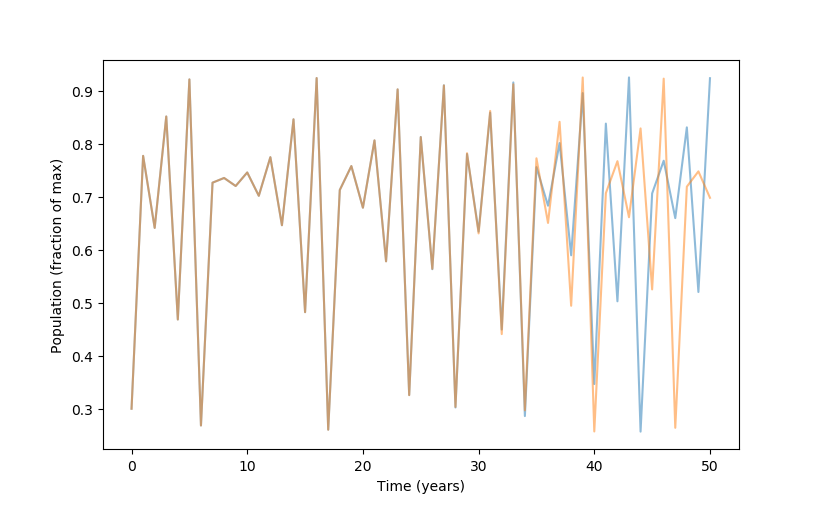
The two trajectories are nearly identical but then diverge. This is sensitivity to initial conditions, and has been shown by Lorenz to be implied by and to imply aperiodicity (more on this below).

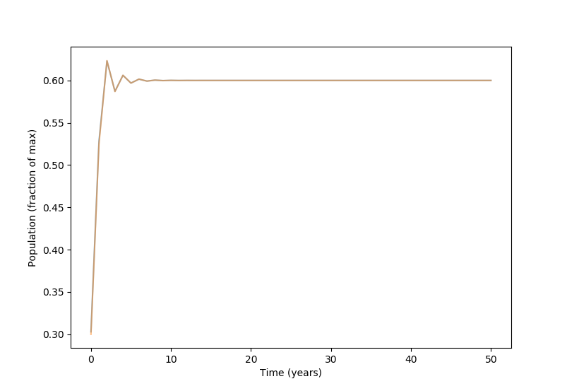
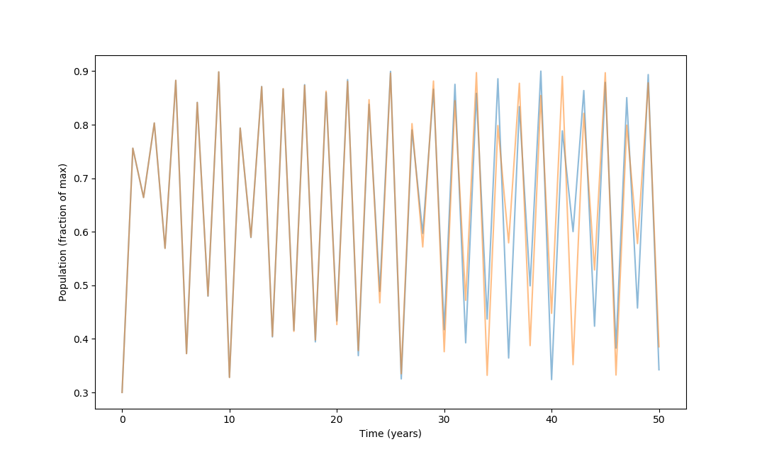
In contrast, a relatively large shift of a factor of one hundreth (3 to 3.03) in initial population leads to no change to periodicity or exact values at $r=2.5$ (period 1):

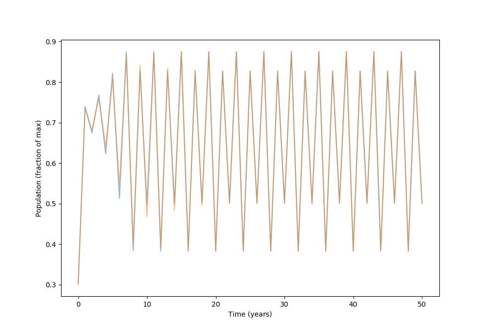
or at $r=3.5$, period 4, the same change does not alter the pattern produced:

even a large change in starting value at $r=3.55$ (period 8), from $x_0=0.3$ to $x_0=0.5$ merely shifts the pattern produced over by two iterations but does not change the points obtained or the order in which they cycle:

Patterns in the aperiodic orbit map

Information from iterating \eqref{eq1} at different values of $r$ may be compiled in what is called an orbit map, which displays the stable points at each value of $r$. These may also be though of as the roots of the equation with specific $r$ values.

To do this, let’s have the output of the logistic equation on the y-axis and the possible values of $r$ on the x-axis, incremented in small units.

#Import third-party libraries
import numpy as np 
import matplotlib.pyplot as plt 

def logistic_map(x, y):
	'''a function to calculate the next step of the discrete map.  Inputs
	x and y are transformed to x_next, y_next respectively'''
	y_next = y * x * (1 - y)
	x_next = x + 0.0000001
	yield x_next, y_next

For high resolution, let’s use millions of iterations. Note that the logistic equation explodes to infinity for $r > 4$, so starting at $r = 1$ let’s use 3 million iterations with step sizes of 1/100,000 (as above)

steps = 3000000

Y = np.zeros(steps + 1)
X = np.zeros(steps + 1)

X[0], Y[0] = 1, 0.5

# map the equation to array step by step using the logistic_map function above
for i in range(steps):
	x_next, y_next = next(logistic_map(X[i], Y[i])) # calls the logistic_map function on X[i] as x and Y[i] as y
	X[i+1] = x_next
	Y[i+1] = y_next

Let’s plot the result! A dark background is used for clarity.

lt.style.use('dark_background')
plt.figure(figsize=(10, 10))
plt.plot(X, Y, '^', color='white', alpha=0.4, markersize = 0.013)
plt.axis('on')
plt.show()

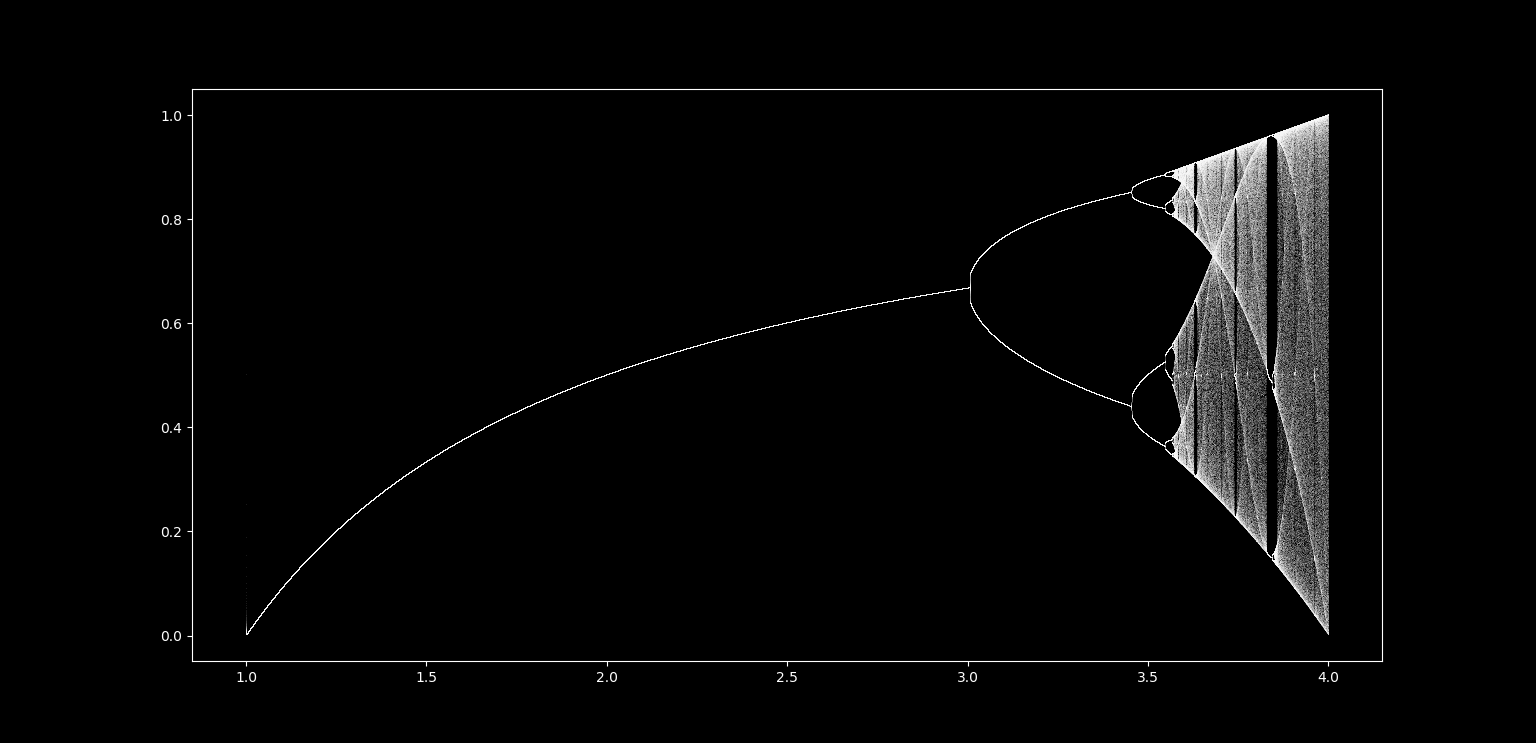
By looking at how many points there are at a given $r$ value, the same patter of period doubling may be observed. The phenomenon that periodic nonlinear systems become aperiodic via period doubling at specific ratios was found by Feigenbaum to be a near-universal feature of the transition from periodicity to chaos.

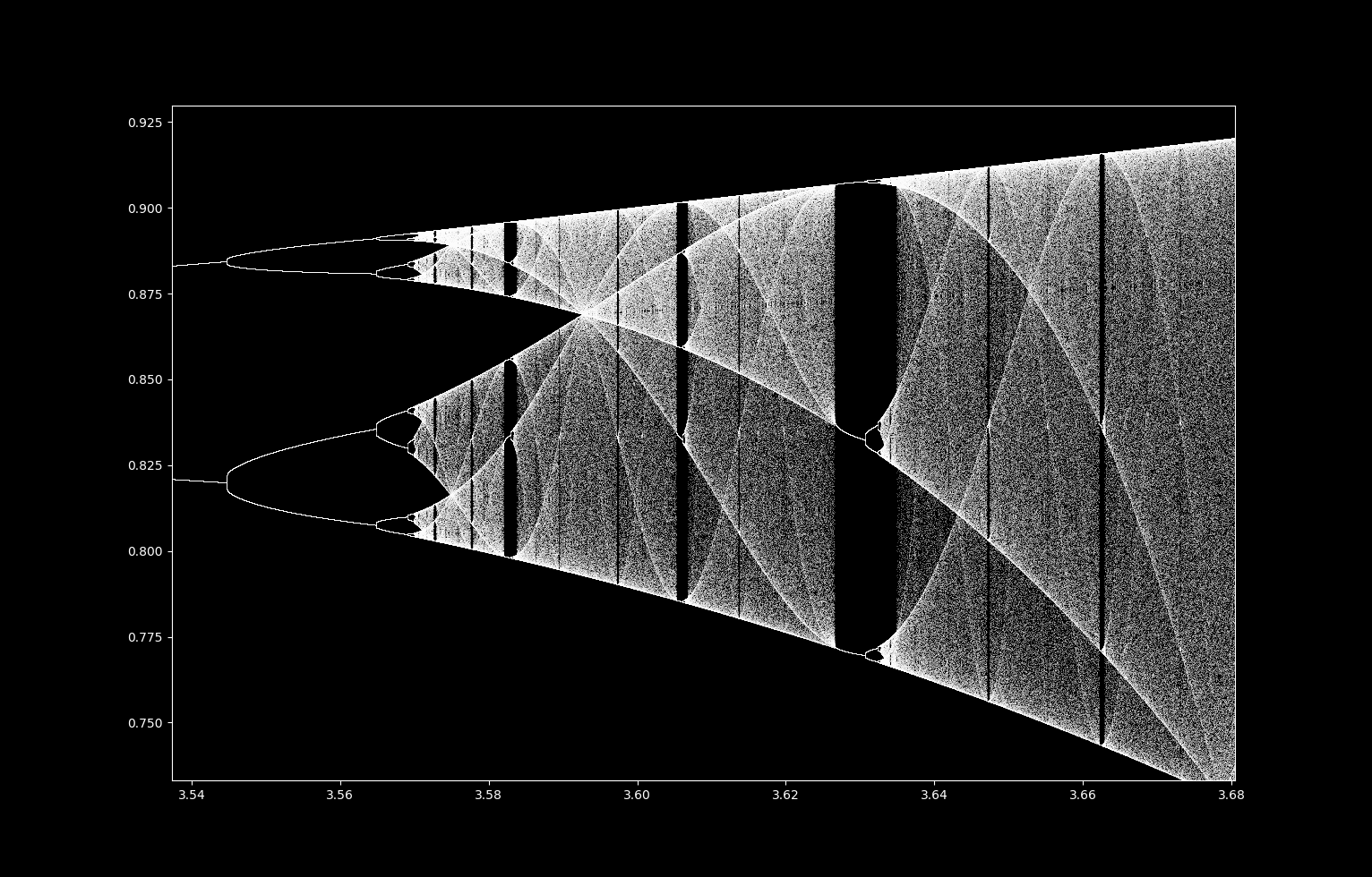
Let’s take a closer look at the fuzzy region of the right. This corresponds to the values of $r$ which are mostly aperiodic, but with windows of periodicity. There are all kinds of interesting shapes visible even in the aperiodic sections:

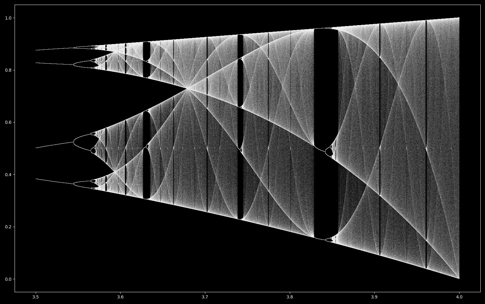
What do these shapes mean? It is worth remembering what this orbit diagram represents: a collection of single iterations of \eqref{eq1} with very slightly different $r$ values, the previous iteration population size being the input for the current iteration. This is why the chaotic regions appear to be filled with static: points that are the result of one iteration of the logistic equation are plotted, but the next point is mostly unpredictable and thus may land anywhwere within a given region. The shapes, ie regions of higher point density, are values that are more common to iterations of changing $r$ values.

Are these same values more common if $r$ is fixed and many iterations are performed at various starting population size values? Let’s take $ r \approx 3.68$, where the orbit diagram exhibits higher point density at population size $p \approx 0.74$. THe proportion of iterations near each value may be plotted in R,

# data taken from 900 iterations of the logistic equation starting at 3, 6, and 9 (+ 0.0000000000000001) at r=3.68
library(ggplot2)
data1 = read.csv('~/Desktop/logistic_0.3_4.csv', header=T)
a <- ggplot(data1, aes(value))

a + geom_dotplot('binwidth' = 0.01, col='blue', fill='red') +
    xlim(0, 1) +
    theme_bw(base_size = 14) 

Here the x-axis denotes the population size, and the y-axis denotes the proportion of iterations in this region:

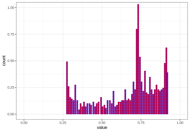
and thus there are are indeed more iterations near $0.74$ than elsewhere, holding $r$ constant and iterating from a few different starting points.

Why are certain points more common than others, given that these systems are inherently unpredictable? Iterating \eqref{eq1} at $r=3.68, x_0=0.3$ as shown above provides a possible explanation: the population only slowly changes if it reaches $x \approx 0.728$ such that many consecutive years (iterations) contain similar population values.

Each point in the aperiodic logistic map’s trajectory is unstable, meaning that every value arbitrarily close to the point of interest will eventually become arbitrarily far away (within the bounds of the function’s image). But these numerical test suggest that points near $0.7282…$ move comparatively less than others.

Fixed points for $r=3.68$ may be found:

\[x_n = rx_n(1-x_n) \\ x_n = 0, x_n = 0.728261\\\]

Note that our relatively stable point above is very close to the (unstable) point of period 1. These points have linear stabilities of

\[f'(0) = 3.86\\ f'(0.72826) = -1.68\]

Now $\lvert -1.68 \rvert > 1$ and so the point is unstable, but note that it is not very unstable as it is close to 1. This means that subsequent iterations will diverge, just slowly, which explains why points near $x_n=0.7282…$ tend to have subsequent iterations near their current value.

This does not really explain why these points are more likely to be visited by any trajectory because points of every periodicity are possible, not just period 1. To address this, one can ask how stable is this point compared to (unstable) points of other periodicities. For period two points,

\[x = 0, \; x \approx 0.39, \; x \approx 0.72, \; x \approx 0.87 \\ (f^2(0))' = -113.2145 \\ (f^2(0.393))' = -79.06 \\ (f^2(0.728))' = -31.63 \\ (f^2(0.878))' = −17.61 \\\]

But as there are infinitely many periodic points, this approach is flawed because we will never be done comparing stabilities at different points. Instead, the following technique presented by Strogatz uses a geometric analytic argument: where does $x_{n+1}$ change the least for any given change in $x_n$? This occurs near $x_n = 0.5$, as the absolute value of derivative of the logistic map $f’(x) = r(1-2x)$ is minimized when $x=1/2$. Therefore the most stable $x_n$ values exist for iterations following this value.

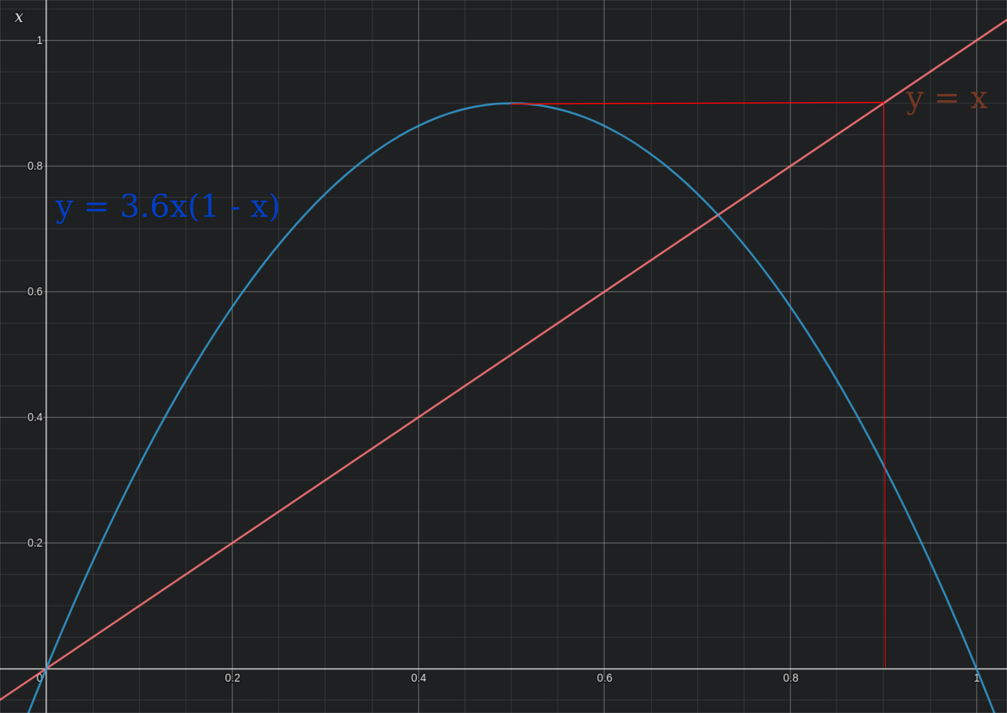
This is best seen using a cobweb plot, which plots the equation of interest (here $rx(1-x)$) and the line $y=x$ in order to follow iterations geometrically. The principle is that $y=x$ is used to reflect y-values onto the x-axis, thereby allowing iterations to be plotted clearly. The procedure is as follows: given any point on the x-axis, find the y-value that corresponds to $rx(1-x)$. This is the value of the next iteration of \eqref{eq1}, and this value is reflected back onto the x-axis by travelling horixontally until the $y=x$ line is reached. The x-value of this point is the same as the y-value we just found, and therefore we can repeat the process of finding a subsequent iteration value by again finding the y-value of the curve $rx(1-x)$ and travelling horizontally to meet $y=x$.

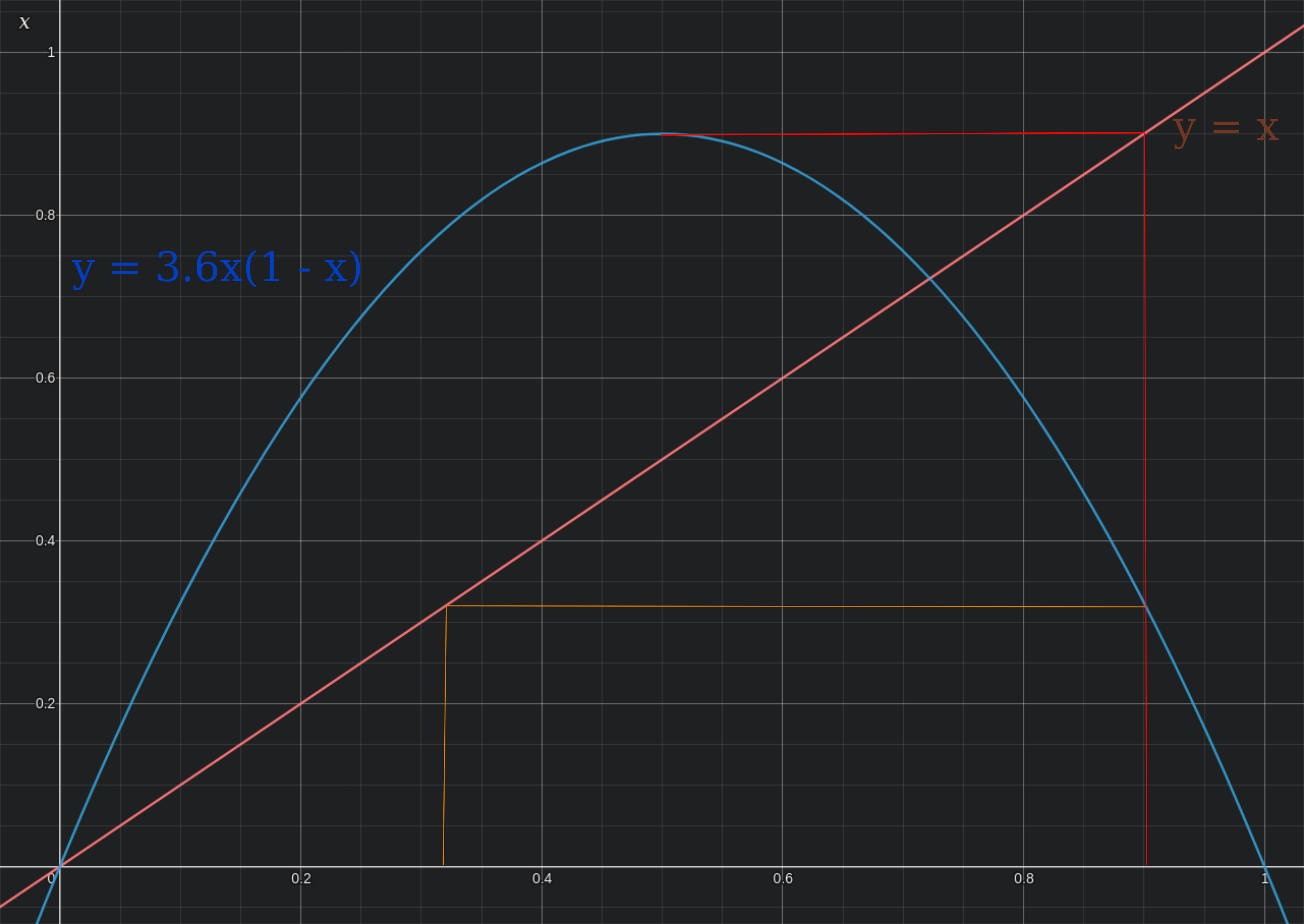
For example, if $r=3.6$, $x_n = 0.5$ gives $x_{n+1} \approx 0.91$.

and another iteration gives $x_{n+2} \approx 0.32$,

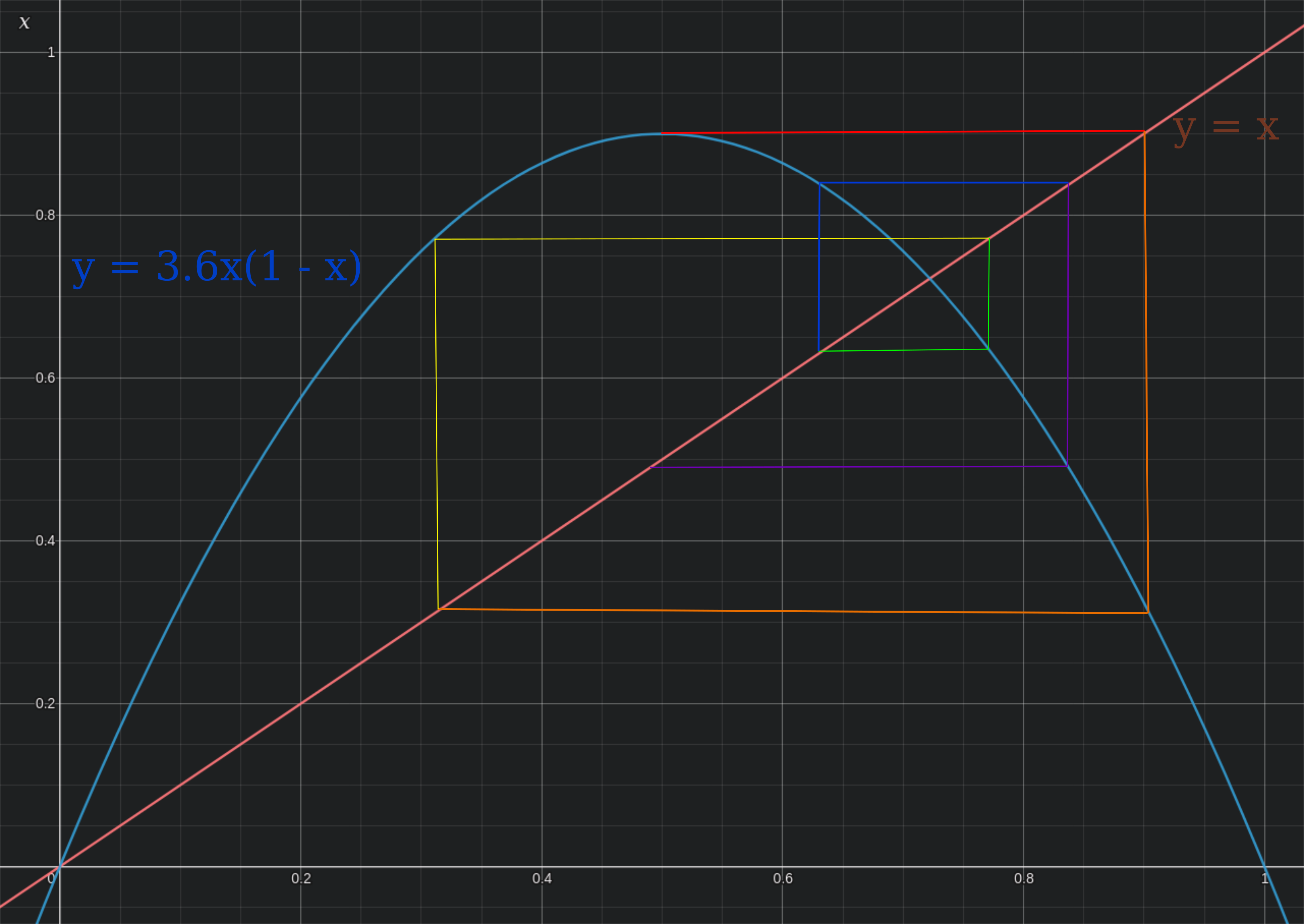
After six iterations (red, orange, yellow, green, blue, indigo respectively), there is

Now as one ranges over r values, the first four iterations after $x_n=0.5$ are in red, yellow, green, and blue respectively:

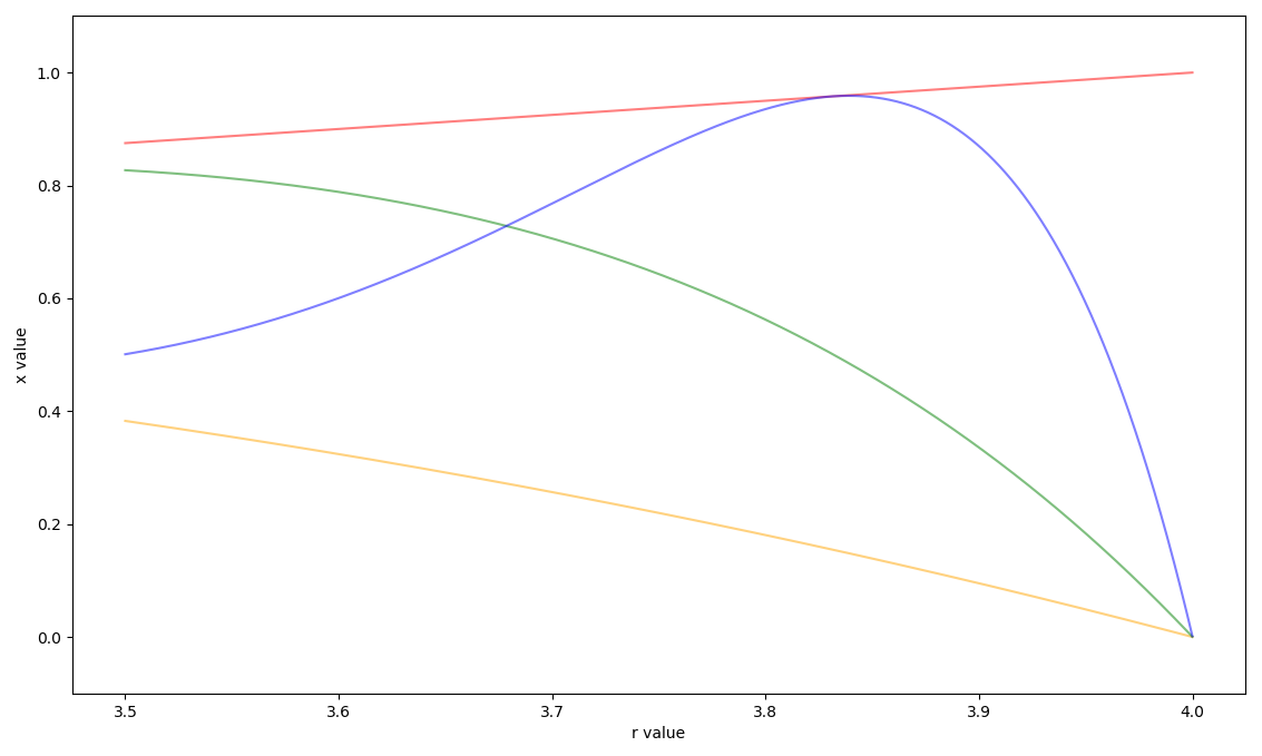
Overlayed onto the logistic map with successive iterations after $x_n=1/2$ in red, orange, yellow, green, blue, indigo, and violet respectively,

Aperiodicity with sensitivity to initial values, also called mathematical chaos, results when points are everywhere unstable. But as this section has demonstrated, they are not necessarily equally unstable everywhere which illustrates a feature of chaos that differs from its English usage: mathematical chaos is not completely disordered. A more descriptive word might be ‘mysterious’ because these systems are unpredictable, even if they are partially ordered or are bounded by spectacular patterns, as seen in the following section.

This phenomenon of patterns arising amidst aperiodicity is also found in prime gaps.

Prediction accuracy

Consider the logistic map for, $r = 3.6$ and $r = 4$. In contrast to complete disorder, short-range prediction is possible with chaotic systems even if long-range prediction is impossible. Does relatively restricted aperiodicity (as seen for $r=3.6$) lead to an extension in prediction range? Let’s compare iterations of two starting values at a factor of a ten-thousanth apart (0.3 and 0.30003) to find out:

$r=3.6$

$r=4$

Observe that the divergence in values occurs later for $r=3.6$ than for $r=4$, implying that longer-range prediction is possible here. Iterations of \eqref{eq1} at both values of $r$ are chaotic, but they are not equally unpredictable.

To illustrate this more clearly, here is a plot of the first iteration of divergence (100 iterations mazimum) of \eqref{eq1} at varying $r$ values, with $p_{01} = 3, p_{02} = 3.0003$.

To do this, the first step is to initialize an array to record $r$ values from 3.5 to 4, taking 500 steps. The next step is to count the number of iterations it takes to diverge (with a maximum interation number of 100 in this case). Arbitrarily setting divergence to be a difference in value greater than 0.15,

steps = 500
y = np.zeros(steps + 1)
r = np.zeros(steps + 1)
r[0] = 3.5
y[0] = 100

for i in range(500):
	X1 = 0.3
	X2 = 0.3 + 0.3**(t/30)

	for j in range(100):
		X1 = r[i] * X1 * (1-X1)
		X2 = r[i] * X2 * (1-X2)

		if np.abs(X1 - X2) > 0.15:
			break

	y[i+1] = j + 1
	r[i+1] = r[i] + 0.001

which when plotted yields

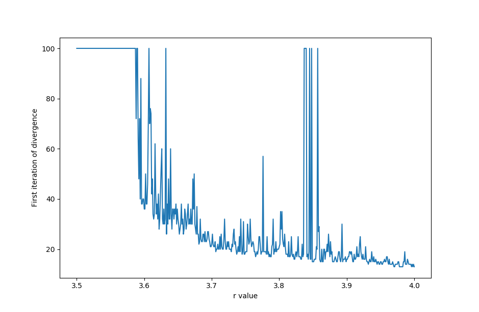
Prediction ability (in length until divergence) tends to decrease with increasing $r$ values, but the exact relationship is unpredictable: some small increases in $r$ lead to increased prediction ability.

Increasing the accuracy of the initial measurement would be expected to increase prediction ability for all values of $r$ for \eqref{eq1}. Is this the case? Let’s go from $\Delta x_0 = 1 \to \Delta x_0 \approx 3.5 \times 10^{-11}$.

Thus prediction power does increase with better initial measurements, but not always: the benefit is unpredictable. Notice that for certain values of $r$ the number of iterations until divergence actually increases with a decrease in $\Delta x_0$: this means that paradoxically increased accuracy can lead to decreased prediction accuracy!

Ranging $r=3.5 \to r=4$, small changes in $r$ lead to little change to iterations of \eqref{eq1} with $x_0 = 0.3$ if the trajectory is periodic. But when aperiodic, small changes in $r$ lead to large changes in the population trajectory.

This sensitivity to constant values as well as initial population is important because in the real world, no measurement is perfect but is merely an estimation: the gravitational constant is not 9.8 meters per second squared but simply close to this value. Necessarily imperfect measurements mean that not only would one have to take infinitely long to predict something at arbitrarily (infinitely) far in the future, but beyond a certain point the predictions will be inaccurate.

This was first shown in Lorenz’s pioneering work mentioned above, in which a deterministic model of air convection was observed to exhibit unpredictable behavior. A simplified proof for the idea that aperiodicity implies sensitivity to initial values, based on Lorenz’s work, is found here.

Nonlinear maps are often fractals

One of the most striking features of this map is that it is a self-similar fractal. This means that smaller parts resemble the whole object. Observe what happens when we zoom in on the upper left section of the aperiodic region in the logistic map: A smaller copy of the original is found.

If we take this image and again zoom in on the upper left hand corner, again we see the original!

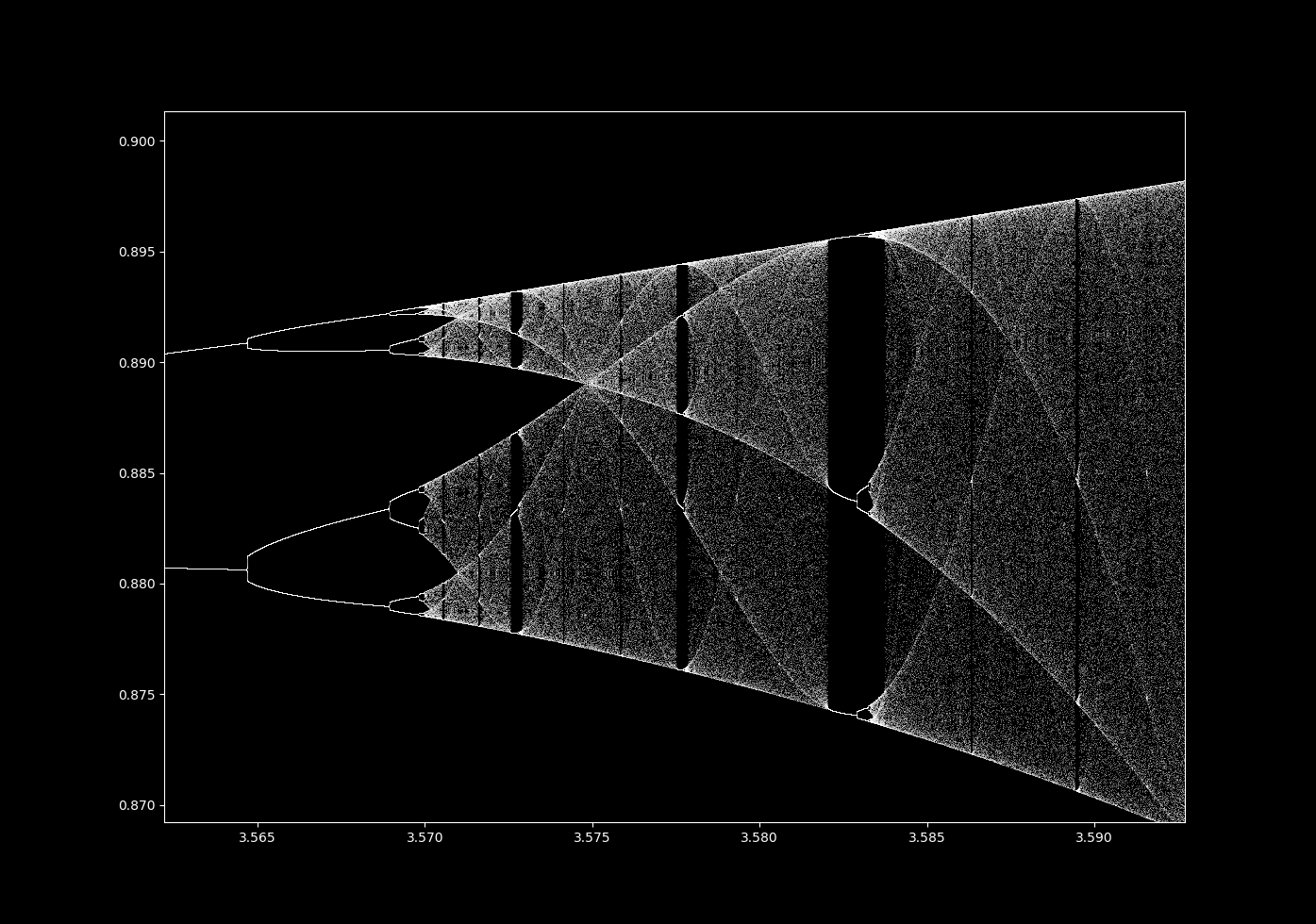
Zooming in by a factor of $2^{15}$ on the point $(3.56995, 0.8925)$, we have

An infinite number of smaller images of the original are found with increasing scale. Far from being unusual, the formation of fractals from nonlinear systems is the norm provided that they are dissipative and do not explode towards infinity nor exhibit a point or line attractor.

Period three

As $r$ increases, the periodicity increases until it becomes infinite, and infinite periodicity is equivalent to aperiodicity. This occurs via period doubling: as can be seen clearly from the logistic map, one period splits into two, which split into four, which split into eight etc. This period doubling occurs with less and less increase in $r$ such that an infinite period is reached within a finite increase in $r$, and at this point the map is aperiodic. This occurs whenever there is a transition from periodicity to aperiodicity.

Looking closely at the orbit map, it seems that there are regions where an aperiodic trajectory transitions into a periodic one, for example at around $x = 3.83$ where there are three values where that $f(x)$ is located. Is this really a transition away from aperiodicity?

For $r=3.83$, most initial values in $(0.3, 0.8)$ when iterated with the logistic map are numerically attracted to the following period 3 orbit:

\[0.50466649, \; 0.9574166, \; 0.15614932, \; 0.50466649 ...\]

Checking that these points are indeed prime period 3 is a task of finding the roots of $f^3(x) = x$ when $r = 3.83$. $f^3(x)$ is the rather complicated expression

\[f^3(x) = -r^7x^8 + 4r^7x^7 \\ - (6r^7+2r^6)x^6 + (4r^7+6r^6)x^5 \\ - (r^7+6r^6+r^5+r^4)x^4 \\ + (2r^6 + 2r^5 +2r^4)x^3 \\ -(r^5 + r^4+r^3)x^2 + r^3x \\\]

so finding the solutions to $f^3(x)-x = 0$ is best done using a computer algebra evaluator, which yields

\[0 \approx -12089.028955x^8+48356.11582x^7 \\ -78846.982583x^6+67294.542381x^5 \\ -32066.758626x^4+8391.415073x^3 \\ -1095.484996x^2+55.181887x\]

This is a greater-than fourth order equation, meaning that there is no formula akin to the quadratic or cubic formulas that allow us to evaluate roots. Instead roots can be found using an analytic technique, such as Newton’s or Halley’s method. Using Halley’s method (code here) and selecting for real roots between 0 and 1, there is

[(0.504667), (0.16357), (0.156149), (0.524), (0.738903), (0), (0.957418), (0.955293)]

Each of the points found numerically are found, along with five others. The stability of each point may be checked by evaluating $abs (f^3(x))’ < 1 $, which can be done using the program above, which results in the ungainly equation

f^3(x). = -96712.23164x^7+338492.81074x^6-473081.895498x^5+336472.71190500003x^4-128267.034504x^3+25174.245219x^2-2190.969992x+56.181887

Evaluating this equation with class Calculate gives, respectively,

[0.329918, 1.652343, 0.329823, 1.652285, -6.12846, 56.181887, 0.328975, 1.652814]

and this means that as expected, only the roots that were attractors in the numerical approach are stable, and the rest are unstable. As an aside, note that the root at 0 has the largest value of $(f^3)’(x)$, and numerically is the most unstable of all points.

But there is something different about $r=3.83$ that yields (prime) period 3 points compared to those observed above for prime period 1 or 2. Let’s try to find points of period 4, which involves finding the roots of the equation $f^4(x) - x = 0$ which for $r=3.83$ is the unfortunate

-559733898.714433x^16+4477871189.715462x^15-16257127648.301172x^14+35437147718.087624x^13-51706394045.119659x^12+53298583067.632263x^11-39921349801.953377x^10+22008774729.800488x^9-8946369923.674864x^8+2660008486.237636x^7-568040584.628146x^6+84473618.951678x^5-8330423.126762x^4+503584.653117x^3-16284.736485x^2+214.176627x

which Halley’s method estimates real roots at

[(0.60584), (0.738903), (0.803014), (0.299162), (0.369161), (0), (0.891935), (0.914596)]

Some of these points are not prime period 4, but rather prime period 1 or 2. But some (eg. x = 0.2991621) are truly prime period 4, which is suprising indeed! How can there be prime period points of period 4, given that we already found points of prime period 3 and 4 is greater than 3?

This observation is not specific to the logistic map: any (discrete) dynamical system of a continuous function with period 3 also contains (unstable) points of every other integer period. This means that if period 3 is observed, one can find unstable trajectories of period 5, period 1, period 4952 and so on. This result is due to Sharkovskii, who found the complete order on the integers:

\[3, \; 5, \; 7, \; 9, \; 11, ... \\ 6, \; 10, \; 14, \; 18, \; 22, ... \\ 12, \; 20, \; 28, \; 36, \; 44, ... \\ \vdots \; \; \\ ... 16, \; 8, \; 4, \; 2, \; 1\]

where any prime period also gives points of prime period for any number to the right or bottom of the first.

As observed by Li and Yorke, period three also implies an uncountably infinite number of (unstable) aperiodic trajectories.

Exits from aperiodicity

The conclusion from the last section is that for values of $r$ of the logistic map such that there is a period-3 orbit, there are simultaneously orbits of any finite period as well as infinite-period (which are by definition aperiodic) orbits for this same $r$ value. These are unstable, whereas the period-3 orbit is stable which is why we see points attracted to this particular orbit.

Now consider the transition from an area in the orbit map where no orbit is stable (and thus the trajectory is aperiodic) to an an area of a stable period-3 orbit (but still with points of aperiodicity, albeit unstable ones). Here is a closer view at the transition to period 3 near $r=3.8285$ (right click to view image in higher resolution):

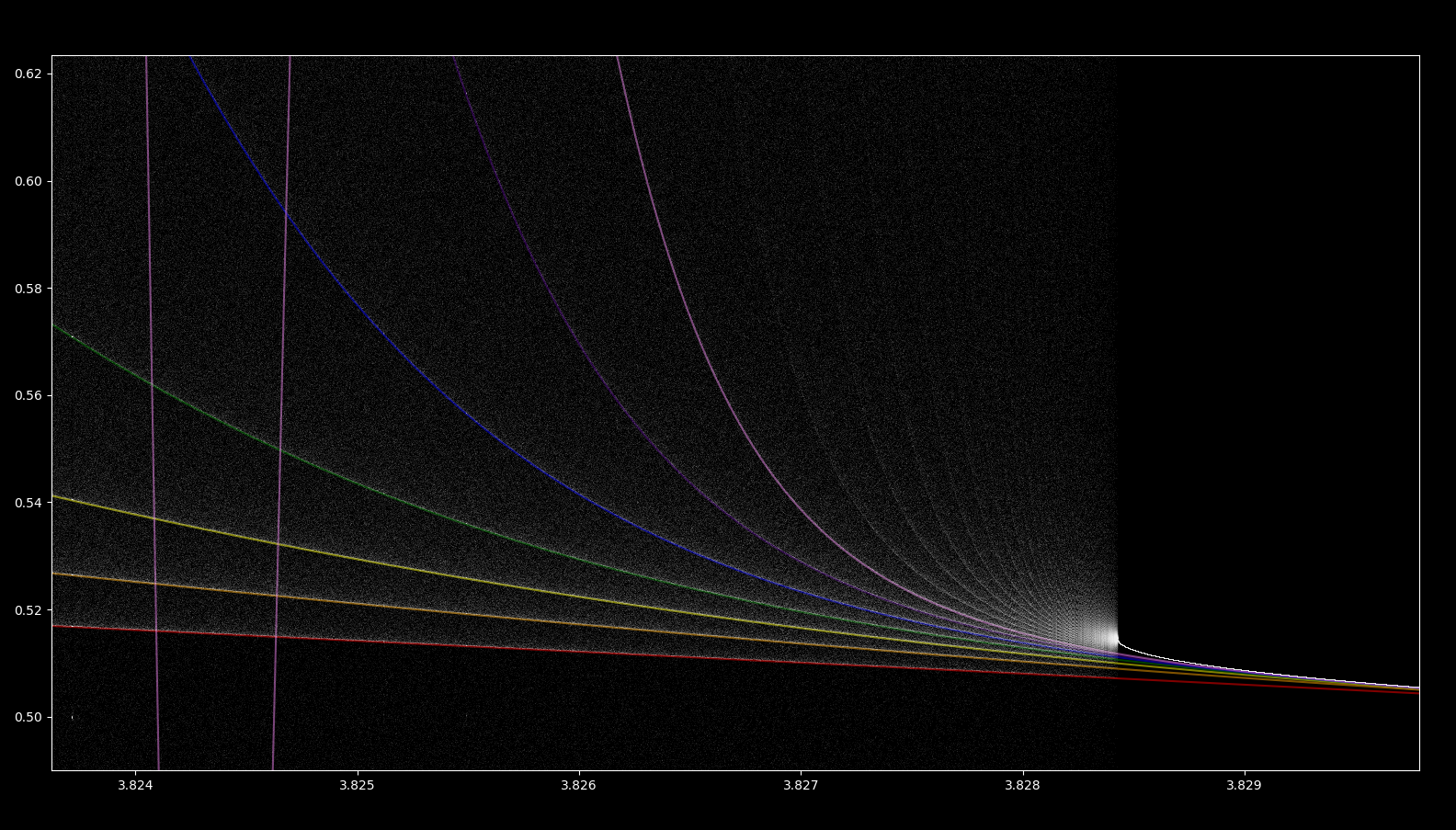
Every third iteration of the logistic map starting from the relatively stable point of $x_0=1/2$, ie

\[x_3, x_6, x_9, x_{12}, x_{15}, x_{18}, x_{21}\]

is also added and color coded as red, orange, yellow, green, blue, indigo, and violet respectively. There are three points of period 3 near $r=3.83$, and so a third of all iterations from $x_0 = 1/2$ go to each point.

Here we see that every third iteration from $x_0 = 1/2$ is less unstable than the surrounding points, and so each has a higher point density. The iterations approach one another as $r$ increases until they meet at around $r=3.82$. A quick look at the logistic map suggests that the meeting of less-unstable points, particularly a meeting where these points approach at a decreasing rate (ie $\frac{d}{dr}x_3 - x_0 \to 0$) occurs for practically all transitions from aperiodicity to periodicity, whatever the period (3, 5, 7, 6, 12, etc.)

Does a meeting of iterations of $x_0 = 1/2$ necessarily lead to a transition from aperiodicity to periodicity? Yes, and here is why:

First note that if two points $f(x_0), f^k(x_0), k > 2$ approach one another, then another point $f^{2k}(x_0)$ will also approach because $f(x_0)$ is near-periodic with period $k$. This means that, for the region mapped above, there are not only 7 but really a countably infinite number of less-unstable points that approach one another, and all are iterations from $x_0 = 1/2$ (and therefore orbits from this starting value). There are a countably infinite number of periodic orbits possible (see here for more on this), and therefore there are as many possible periodic orbits as there are less-unstable orbits that converge. Then the value the less-unstable orbits converge upon becomes stable with respect to those periodic orbits because they are all accounted for.

Now note that all points plotted using any computer are, strictly speaking, periodic: there are only so many possible values because computers use finite decimal precision. Therefore eventually all values repeat: thus each point plotted is really a member of a periodic orbit. As there are countably many periodic orbits possible and as countably many periodic orbits converge whenever two or more meet, the convergence value becomes stable for points that are plotted by a computer.

Orbit map revisited

It is interesting to consider what the logistic orbit map represents: periodic points that are stable, not periodic points that are unstable. With very accurate arithmetic, the logistic map looks quite different.

This can be plotted using the Decimal class in python, which implements arbitrary (within memory bounds, that is) decimal precision arithmetic. For a constant $300000$ steps starting at $r=2.95$ and ending at $r=4$, increasing from $8$ to $28208$ digits of decimal precision yields

And with perfect precision, the orbit map would display only the points that are periodic at the start: an orbit map beginning at $r=0$ with a periodic point at $x_n=0$ would remain at $x_n=0$ throughout (until $r>4$). An orbit map starting at $r=1$ would retain a period 1 attractor for the orbit map, which can be modeled by increasing decimal accuracy from 8 to 5587 digits, $r \in [1, 4]$, with 100000 steps as follows:

And an orbit map starting at period 2 would remain in period 2, and the same for 4, 8, etc.

But what would happen if we began the orbit map in the aperiodic region $r > 3.56995…$, assuming we had the ability to perfom infinite precision arithmetic? If one were able to calculate with perfect precision, what would the orbit map look like? Clearly a substantial change would occur in the periodic windows in the aperiodic region, because these periodic windows are stable orbits that coexist with many unstable ones. With perfect precision, iterations in any of these unstable orbits would remain in that orbit rather than head to a stable point.

For example, earlier in this page it was found that the (stable) period three region at $r=3.83$ also exhibited a period 4 trajectory that contains $x_n = 0.2991621…$. This means that if one were to begin iterating at this point with perfect precision, the orbit map would exhibit a period 4 region for $r=3.83$ instead. From Sharkovskii’s total order above, this is also true for any other integer in this period three region: given any desired period, we can find a point such that $r=3.83$ exhibits a period of that value there.

This is not all: from Sharkovskii’s as well as Li and Yorke’s work, it is shown that there are uncountably many unstable aperiodic orbits for period 3 (or 6 or 12 or 5…), it follows that nearly all trajectories in the aperiodic region are unstable but aperiodic. With perfect precision, instability is irrelevant and therefore most trajectories through these regions would remain aperiodic. Thus if one were to pick a value ($x_0 \in \Bbb R$ and in the domain of the logistic map) at random for the period three region $r=3.83$ (or any aperiodic region $r> 3.565995…$), it is almost certain to exist on an aperiodic but unstable trajectory such that the periodic windows we see with the orbit map would no longer be visible.

Exact solution for r=4

At r=4, the logistic map exhibits a fascinating conjuction of properties: aperiodicity with solvability. By this is meant that we can express the location of any future point $x_{n+a}$ in a closed form, non-recursive expression: we no longer need to iterate \eqref{eq1} in order to find out where a future iteration will be. And yet this map is also aperiodic, and furthermore it is sensitive to initial conditions such that any arbitrarily close $x_0, x_{0’}$ will eventually diverge given enough iterations.

The relationship between solvability and aperiodicity, which are intuitively opposing ideas, is explored elsewhere.