Three body problem II: Simulating Divergence with Parallelized Computation

This page is a continuation from Part 1, where simulations of the three body problem are explored. Here we explore the computation of simulated trajectories using a parallelized computer achitecture, ending with am optimized CUDA kernal that is around five times as fast as the Pytorch code introduced in Part 1.

Introduction

Most nonlinear dynamical systems are fundamentally irreducible: one cannot come up with a computational procedure to determine the parameters of some object at any given time in the future using a fixed amount of computation. This means that these systems are inherently sequential to some extent. This being the case, there are still many problems that benefit from computations that do not have to proceed in sequence. One particular example is the problem of finding which positions in a given plane are stable for the trajectory of three bodies in space. This problem can be approached by determining the stability of various starting locations in sequence, but it is much faster to accomplish this goal by determining the stabilities at various starting locations in parallel. In Part 1 this parallel computation was performed behind the scenes using the Python torch library, which abstracts away the direct computation of tensors on parallelized computational devices like graphics processing units (GPUs) or tensor processing units.

Even with the use of the optimized torch library, however, computation of stable and unstable locations takes a substantial amount of time. Most images displayed in part 1 require around 18 minutes to compute: this is due to the large number of iteration required (50,000 or more), the large size of each array (18 arrays with more than a million components each) and even the data type used (double precision 64-bit floating point).

A CUDA kernal for divergence

Here we will explore speeding up the three body computation by writing our own GPU code, rather than relying on torch to supply this when given higher-level instructions. The author has an Nvidia GPU and code on this page will therefore be written in C/C++ CUDA (Compute Unified Device Architecure). The code contains a standard C++ -style library inclusion and function initialization (C or C++ execution always begins with main()), all of which is performed on the CPU. Here we first initialize some constants for the three body similation.

#include <stdio.h>
#include <iostream>
#include <chrono>

int main(void)
{
  int N = 90000;
  int steps = 50000;
  double delta_t = 0.001;
  double critical_distance = 0.5;
  double m1 = 10;
  double m2 = 20;
  double m3 = 30;

And then we continue by assigning pointer variables with the proper data type for each of our planets. This is an efficient form of an array in C++, allowing us to allocate memory and initialize each element directly.

In the above code snippet N is the number of pixels; for example a 300x300 divergence plot contains N=90,000 pixels. We will perform all the required computations in 1D arrays for now, such that separate arrays are initialized for each x, y, z component of each attribute of each planet. Note however that this is purely for the purpose of clarity: we could just as easily maintain one single triply large array for all three x, y, z components and instead offset each component by a factor of 1/3 times the size of the array.

We also have to initialize position, acceleration (dv), velocity, and a temporary buffer array for new velocities as shown below.

int main(void)
{
  ...
  double *p1_x, *p1_y, *p1_z;
  ...
  double *dv_1_x, *dv_1_y, *dv_1_z;
  ...
  double *nv1_x, *nv1_y, *nv1_z;
  ...
  double *v1_x, *v1_y, *v1_z;

We also want to initialize boolean arrays for trajectories that have not diverged yet for any given iteration, a boolean array for trajectories that are not diverging right now, and an array to keep track of the iteration in which divergence occurred.

bool *still_together,*not_diverged;
int *times

For each array, we must allocate the proper amount of memory depending on the type of data stored. We have $N$ total elements, so we need to allocate the size of each element times $N$ for each array.

  ...
  p1_x = (double*)malloc(N*sizeof(double));
  ...
  still_together = (bool*)malloc(N*sizeof(bool));
  times = (int*)malloc(N*sizeof(int));
  not_diverged = (bool*)malloc(N*sizeof(bool));  

Next, space is allocated for each array in the GPU. One way to do this is to declare a new pointer variable corresponding to each array (see below for p1_x) before allocating the proper amount of memory for that variable (which must be referenced as it was defined as a pointer. Each must be different than the name for each corresponding CPU array, and here d_ is prefixed to designate that this is a ‘device’ array.

double *d_p1_x;
cudaMalloc(&d_p1_x, N*sizeof(double)); 

Now we need to initialize each array with our starting condition. As we are working with 1D arrays rather than the 2D arrays, we need to initialize each array to capture 2D information in 1D array. Our approach will be similar to how 2D CUDA arrays are represented in GPU memory, and is sometimes termed a ‘row-major’ layout (as each row is contiguous). This is the most commonly used format today, with the column-major layout (contiguous columns) being used in the past by Fortran.

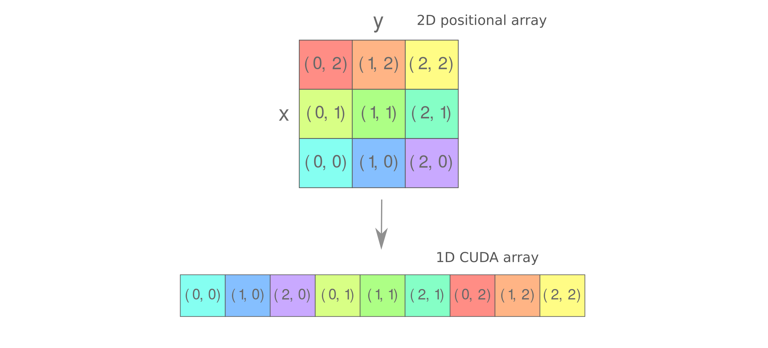
Row-major layout may be implemented using modulo division in which the x parameter is equivalent to the remainder of the division of the total number of elements by the square root of elements, and the y parameter is equal to the integer (floor) division of the number of elements by the square root of elements. Here we also scale each element by the appropriate constants (here to make a linear interpolation between -20 and 20),

  for (int i = 0; i < N; i++) {
    int remainder = i % resolution;
    int step = i / resolution;
    p1_x[i] = -20. + 40*(double(remainder)/double(resolution));
    p1_y[i] = -20. + 40*(double(step)/double(resolution));
    ...

Now we copy each array from the CPU to the GPU

  cudaMemcpy(d_p1_x, p1_x, N*sizeof(double), cudaMemcpyHostToDevice);

and now we can run the CUDA kernal, keeping track of the time spent by initializing a start time clock.

std::chrono::time_point<std::chrono::system_clock> start, end;
start = std::chrono::system_clock::now();
divergence<<<(N+255)/256, 256>>>(
      N, 
      steps, 
      delta_t,
      d_still_together,
      d_not_diverged,
      d_times,
      m1, m2, m3,
      critical_distance,
      d_p1_x,
      ...
      );

CUDA functions are termed ‘kernals’, and are called by the kernal name followed by the number of grid blocks and threads per block for execution. We call our CUDA function by divergence<<<blocks, threads_per_block>>>(args). The denominator of the blocks must equal the threads_per_block for this experiment for reasons detailed below.

We have to synchronize the GPU before measuring the time of completion, as otherwise the code will continue executing in the CPU after the kernal instructions have been sent to the GPU.

  // don't proceed until kernal run is complete
  cudaDeviceSynchronize();
  // measure elapsed kernal runtime
  end = std::chrono::system_clock::now();
  std::chrono::duration<double> elapsed_seconds = end - start;
  std::time_t end_time = std::chrono::system_clock::to_time_t(end);
  std::cout << "Elapsed Time: " << elapsed_seconds.count() << "s\n";

A typical CUDA kernal declaration is __global__ void funcname(args) although __device__ may also be used. For brevity, only the first planet’s arrays are included below but note that the full kernal requires all three planet arrays.

// kernal declaration
__global__
void divergence(int n, 
              int steps,
              double delta_t,
              bool *still_together,
              bool *not_diverged,
              int *times,
              double m_1, double m_2, double m_3,
              double critical_distance,
              double *p1_x, double *p1_y, double *p1_z, 
              double *p1_prime_x, double *p1_prime_y, double *p1_prime_z, 
              double *dv_1_x, double *dv_1_y, double *dv_1_z,
              double *dv_1pr_x, double *dv_1pr_y, double *dv_1pr_z,
              double *v1_x, double *v1_y, double *v1_z,
              double *v1_prime_x, double *v1_prime_y, double *v1_prime_z,
              double *nv1_x, double *nv1_y, double *nv1_z,
              double *nv1_prime_x, double *nv1_prime_y, double *nv1_prime_z,
)

Parallelized computation must now be specified: in the following code, we define index i to be a certain block’s thread, in one dimension as this is how the arrays were defined as well. Note that as the array is 1D, blockDim.x will always evaluate to 1. The arrangement of blocks and threads in our kernal call is now clearer, as each thread is responsible for one index.

{
  int i = blockIdx.x*blockDim.x + threadIdx.x;

Now the trajectory simulation computations are performed. In the spirit of refraining from as much data transfer from the CPU to the GPU and back, we will perform the simulation calculations entirely inside the GPU by moving the trajectory loop to the CUDA kernal. This is notably different than the pytorch approach, where the loop existed on the CPU side (in python) and the GPU was instructed to perform one array computation at a time. It can be shown that moving the loop to the GPU saves a small amount of time, although less than what the author would expect (typically ~5% of runtime with no other optimizations performed).

Moving the loop to the GPU does have another substantial benefit, however: it reduced the electrical power required by the GPU and CPU during the simulation. For the GPU alone, the internal loop typically requires around 100 watts whereas the external loop usually takes around 125 watts on an Nvidia RTX 3060.

For each index i corresponding to one CUDA thread, $steps$ iterations of the three body trajectory are performed and at each iteration the $times$ array is incremented if the trajectory of planet one has not diverged from its slightly shifted counter part (planet one prime).

  for (int j=0; j < steps; j++) {
    if (i < n){
      // compute accelerations
      dv_1_x[i] = -9.8 * m_2 * (p1_x[i] - p2_x[i]) / pow(sqrt(pow(p1_x[i] - p2_x[i], 2) + pow(p1_y[i] - p2_y[i], 2) + pow(p1_z[i] - p2_z[i], 2)), 3) \
                  -9.8 * m_3 * (p1_x[i] - p3_x[i]) / pow(sqrt(pow(p1_x[i] - p3_x[i], 2) + pow(p1_y[i] - p3_y[i], 2) + pow(p1_z[i] - p3_z[i], 2)), 3);
      dv_1pr_x[i] = -9.8 * m_2 * (p1_prime_x[i] - p2_prime_x[i]) / pow(sqrt(pow(p1_prime_x[i] - p2_prime_x[i], 2) + pow(p1_prime_y[i] - p2_prime_y[i], 2) + pow(p1_prime_z[i] - p2_prime_z[i], 2)), 3) \
                    -9.8 * m_3 * (p1_prime_x[i] - p3_prime_x[i]) / pow(sqrt(pow(p1_prime_x[i] - p3_prime_x[i], 2) + pow(p1_prime_y[i] - p3_prime_y[i], 2) + pow(p1_prime_z[i] - p3_prime_z[i], 2)), 3);

      // find which trajectories have diverged and increment *times
      not_diverged[i] = sqrt(pow(p1_x[i] - p1_prime_x[i], 2) + pow(p1_y[i] - p1_prime_y[i], 2) + pow(p1_z[i] - p1_prime_z[i], 2)) <= critical_distance;
      still_together[i] &= not_diverged[i];
      if (still_together[i] == true){
        times[i]++;
      };

      // compute new velocities
      nv1_x[i] = v1_x[i] + delta_t * dv_1_x[i];
      nv1_prime_x[i] = v1_prime_x[i] + delta_t * dv_1pr_x[i];

      // compute positions with current velocities
      p1_x[i] = p1_x[i] + delta_t * v1_x[i];
      p1_prime_x[i] = p1_prime_x[i] + delta_t * v1_prime_x[i];

      // assign new velocities to current velocities
      v1_x[i] = nv1_x[i];

      v1_prime_x[i] = nv1_prime_x[i];
      }
    }

The same needs to be done for all x, y, z vectors of p1, p2, p3 in order to track all the necessary trajectories. In total we have 63 vectors to keep track of, which makes the cuda code somewhat unpleasant to write even with the help of developer tools.

The cuda kernal with driver code can be compiled via nvcc, which is available through the nvidia cuda toolkit. Linux users be warned that the drivers necessary for full Nvidia toolkit use with an Ampere architecture GPU (such as the author’s RTX 3060) may not be compatible with the latest linux kernal version, so downgrading to an older kernal version may be necessary. The author has found that kernal version 5.19.0-45-generic is compatible with recent versions of nvcc, and this can be selected in the ‘advanced options’ of the linux boot menu for Ubuntu 22.04.

Those wishing to compile CUDA code via nvcc should note that there are two CUDA versions in each distribution: the runtime API version and the driver version. The driver version should meet or exceed the runtime API software version, which can be checked by ensuring that the CUDA version displayed in the upper right hand corner of the readout called by entering nvidia-smi in bash meets or exceeds that shown when calling nvcc --version.

Here we compile with the flag -o followed by the desired file name where the compiled binary program will be stored.

(base) bbadger@pupu:~/Desktop/threebody$ nvcc -o divergence divergence.cu

For a 300x300 x,y resolution after the full 50,000 timesteps, we have a somewhat disappointing runtime of

(base) bbadger@pupu:~/Desktop/threebody$ ./divergence
Elapsed Time: 144.3s

Compare this to the Pytorch library version of the same problem (see part 1), which

[Finished in 107.1s]

Pytorch employs some optimizations in its CUDA code, so this difference is not particularly surprising and only indicates that the movement of the loop into the cuda kernal does not offer the same performance benefit as other optimizations that are possible. In future sections we explore methods to optimize the cuda kernal further to achieve faster runtimes for the three body problem than are available using torch.

Getting data from CUDA to Numpy

We can compare the planetary array elements from our CUDA kernal to those found for the torch version to be sure that our kernal’s computational procedure is correct. But what if we want to plot the divergence map generated by our CUDA kernal? For the sake of comparison, let’s say that we want to plot our array using the same color map as was presented in part 1. There are no C++ CUDA libraries (to the author’s knowledge) that implement the Matlab-style mathematical plots that matplotlib does, but that is a python library and cannot be directly applied to C-style arrays.

Thus we want a way to send our C++ CUDA-computed arrays (specifically the *int times array) from CUDA C++ to Python for manipulation and visualization there. Perhaps the most straighforward way of accomplishing this task is to use the versatile ctypes library, which

The use of ctypes can get quite complex, but in this case we can apply this library with only a few lines of code. First we need the proper headers in our .cu file containing the CUDA kernal and driver C++ code.

#! C++ CUDA
#include <cuda.h>
#include <cuda_runtime_api.h>

It should be noted that some standard C++ CUDA libraries (ie <equation.h>) are incompatible with the CUDA runtime API, so some care must be taken in choosing the header files for a project that involves ctypes. Next we leave the kernal the same as before, but change the main function declaration, which was

int main(void)
{...

to a function linker that enforces an identical datatype between C++ and C (as we are using ctypes but are programming in C++ Cuda) with whichever arguments we desire.

extern "C" {
  int* divergence(int arg1, int arg2,...)
  {
    ...
    return times;
  }

where we provide the proper return type (here a pointer to an integer array). This code can be compiled by nvcc and sent to a .so (dynamic library) file with the proper flags:

(base) bbadger@pupu:~/Desktop/threebody$ nvcc -Xcompiler -fPIC -shared -o divergence.so divergence_kernal.cu

where our CUDA kernal is located in divergence_kernal.cu and we are sending the compiled library to divergence.so. Now we can call the divergence function in our .so file using `ctypes as follows:

#! python
import numpy as np
import ctypes
import matplotlib.pyplot as plt 

f = ctypes.CDLL('./divergence.so').divergence

Next we need a pointer of the proper type in order to read the function divergence return, which here is ctypes.c_int as well as any argument types (here integers as well). Integers may be passed as arguments without supplying a type definition but other types (double, float, etc) must be supplied via argtypes definition. We need the array size as well, so for a 300x300 array we specify a pointer to a block 300*300 ints large. Then the file contents can be read into an ctypes object <class '__main__.c_int_Array_90000'>.

dim = 300
f.argtypes = [ctypes.c_int, ctypes.c_int]
f.restype = ctypes.POINTER(ctypes.c_int * dim**2)
arr = f(arg1, arg2).contents

At this point we have arr which is a ctypes object that can be converted to a Numpy array very quickly by a direct cast, and the result may be plotted via Matplotlib as follows:

time_array = np.array(arr)
time_steps = 50000
time_array = time_array.reshape(dim, dim)
time_array = time_steps - time_array
plt.style.use('dark_background')
plt.imshow(time_array, cmap='inferno')
plt.axis('off')
plt.savefig('Threebody_divergence_cuda.png', bbox_inches='tight', pad_inches=0, dpi=410)
plt.close()

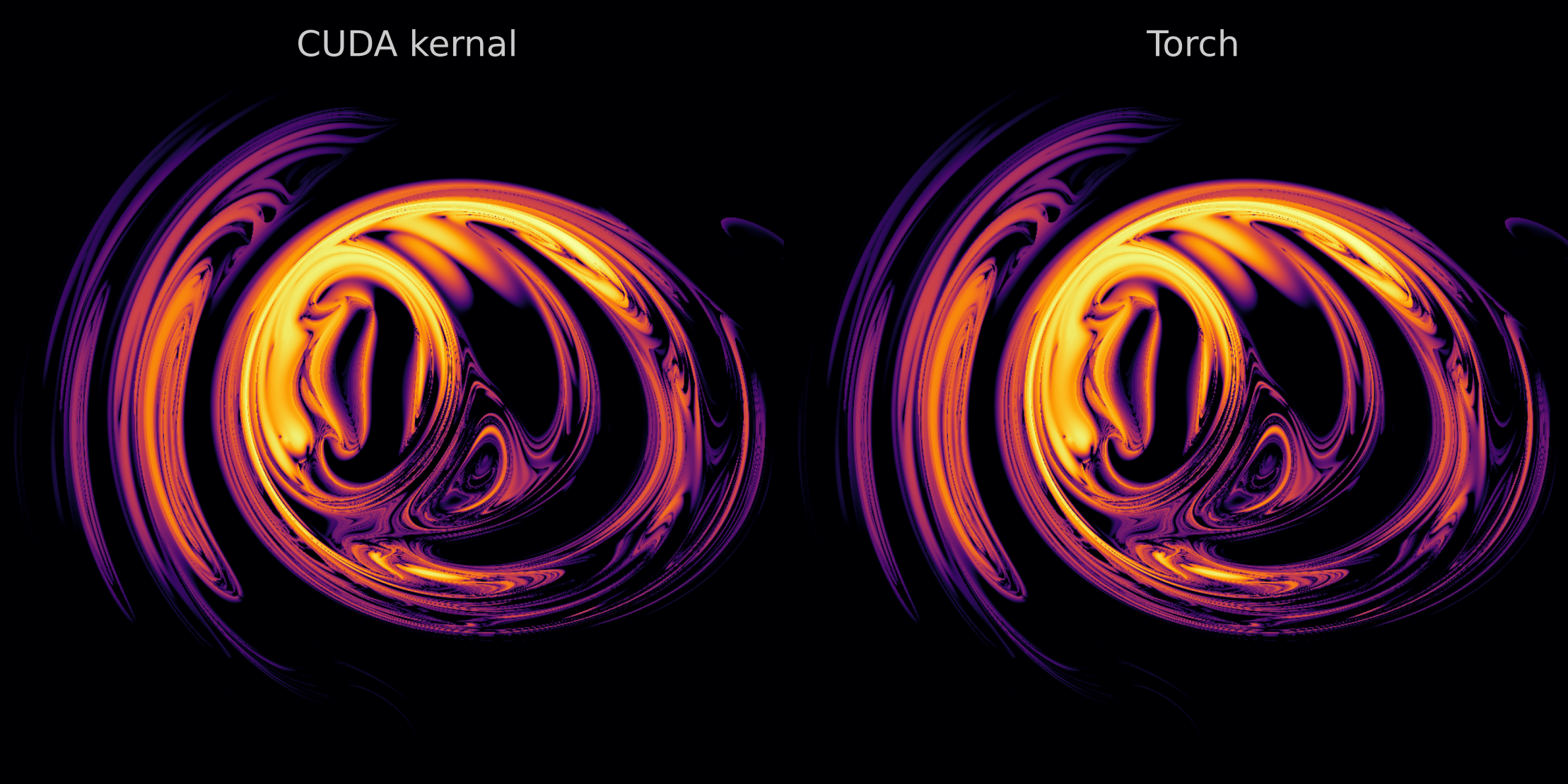
when we compare a 1000x1000 array after 50,000 time steps using our CUDA kernal to the Torch-based calculation, we find that the output is identical (although with optimization the computation time is reduced by a factor of 2.4).

For a write-up on the use of ctypes for cuda-defined functions where Python array arguments are defined and passed to CUDA code, see Bikulov’s blog post.

Optimizing the Three Body Trajectory Computations

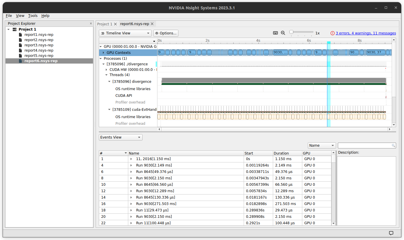
Many data-parallelized programs implemented on GPUs spend more clock cycles (and therefore typically total runtime) on memory management than actual computation. This is nearly always true for deep learning mode inference and also holds for many more traditional graphics applications as well. Memory management occurs both within the GPU and in transfers of data to and from the CPU. For the three body simulation, a quick look at the code suggests that this program should spend very little time sending data to and from the GPU: we allocated memory for each array, initialized each one before sending to the GPU once, and then copied each array back to the CPU once the loop completes. This can be confirmed by using a memory profiler such as Nsight-systems, which tells us that the memory copy from GPU (device) to CPU (host) for the 300x300 example requires only ~20ms. From the screenshot below, it is clear that nearly all the GPU time is spent simply performing the necessary computations (blue boxes on top row).

It may therefore be wondered how much time our kernal spends reading and writing memory within the GPU itself, which for most consumer hardware is one form of vRAM or another. GPUs have a few types of memory, and modern nvidia GPUs typically have what is termed global memory (which is the vRAM storage and is by far the largest form of memory available), shared local memory, and register memory (which was the smallest capacity and is usually reserved for variables). Speed is inversely proportional to the amount of storage the memory element contains, as is the case for different types of CPU memory. In particular, global memory is not actually very fast at all and the idea is that the GPU hides this slow memory access via massive data parallelization.

When arrays (such as double *p1_x) are read or written to the GPU they are by default stored in global memory, which means that we may suspect our kernal as written above to be slower than overwise it perhaps might be because each thread reads and writes many array elements many times over, typically dozens of elements during each iteration. If global memory is indeed accessed at each iteration, it would be expected that changing the memory access pattern to use shared or register elements would drastically speed up the kernal.

Fortunately it is not too hard to change the memory access to register from global memory in the main loop of our CUDA kernal: all we have to do is to assign variables to the proper array elements before the loop commences, and then use only those variables until the loop ends. Variables are by default stored in register memory, so we should not have any global memory access operations if we stick to using only variables in the loop.

// kernal declaration
__global__
void divergence(int n, 
              int steps,
              double delta_t,
              int *times,
	...
	)
{
  int i = blockIdx.x*blockDim.x + threadIdx.x;
  int still_together = 1;
  int not_diverged = 1;
  int times_ind = times[i];
  double p1x = p1_x[i];
  double p1y = p1_y[i];
  double p1z = p1_z[i];
  int times_ind = times[i];
..

This approach has the added benefit of reducing the number of arguments to the void divergence() kernal, as intermediate variable arrays nv1, dv_1_x etc. can be initialized inside the kernal,

double nv1x, nv1y, nv1z;

and in the loop we use these variables to avoid any array read/write operations

  if (i < n){
    for (int j=0; j < steps; j++) {
        // compute accelerations
        dv_1_x = -9.8 * m_2 * (p1x - p2x) / pow(sqrt(pow(p1x - p2x, 2) + pow(p1y - p2y, 2) + pow(p1z - p2z, 2)), 3) \
                 -9.8 * m_3 * (p1x - p3x) / pow(sqrt(pow(p1x - p3x, 2) + pow(p1y - p3y, 2) + pow(p1z - p3z, 2)), 3);

and we can also avoid any if statements in the kernal (branches are typically slow for massively parallelized programming frameworks) as follows:

	// find which trajectories have diverged and increment times_ind
        not_diverged = sqrt(pow(p1x - p1_primex, 2) + pow(p1y - p1_primey, 2) + pow(p1z - p1_primez, 2)) <= critical_distance;
        still_together &= not_diverged; // still_together is initialized as an int with value 0
        times_ind = times_ind + still_together; 

The intermediate variables are updated at each iteration, and at the end of the loop the times_ind value is written to the *times array at the proper location.

 	// compute new velocities
        nv1x = v1x + delta_t * dv_1_x;
	...
        nv1_primex = v1_primex + delta_t * dv_1pr_x;
	...
        // compute positions with current velocities
        p1x = p1x + delta_t * v1x;
	...
        p1_primex = p1_primex + delta_t * v1_primex;
	...
        // assign new velocities to current velocities
        v1x = nv1x;
	...
        v1_primex = nv1_primex;
	...
        }

    times[i] = times_ind;

Running this kernal, however, shows us that there is practically no difference in time saved when we avoid all inner loop array calls. This is because modern CUDA compiler versions optimize memory management for operations like this by default, such that the previously-read array elements are cached in registers without requiring explicit register allocation. This indicates that our kernal is not memory-limitted but instead is compute-limited.

Now that we have convinced ourselves that the three body problem simulation is not memory bandwidth-limited, some experimentation can convince us that by far the most effective single change is to forego use of the pow() cuda kernal operator for simply multiplying together the necessary operands. The reason for this is that the cuda pow(base, exponent) is designed to handle non-integer exponent values which make the evaluatation a transcendental function, which on the hardware level naturally requires many more registers than one or two multiplication operations.

Thus we can forego the use of the pow() operator for direct multiplication in order to optimize the three body trajectory computation. This change makes a somewhat-tedious CUDA code block become extremely tedious to write, so we can instead have a Python program write out the code for us.

def generate_string(a: str, b: str, c: str, d: str, t: str, , m: str, prime: bool) -> str:
    if prime:
        e = '_prime'
    else:
        e = ''
    first_denom =  f'sqrt(({a}{e}_x[i] - {b}{e}_x[i])*({a}{e}_x[i] - {b}{e}_x[i]) + ({a}{e}_y[i] - {b}{e}_y[i])*({a}{e}_y[i] - {b}{e}_y[i]) + ({a}{e}_z[i] - {b}{e}_z[i])*({a}{e}_z[i] - {b}{e}_z[i]))' 
    second_denom = f'sqrt(({c}{e}_x[i] - {d}{e}_x[i])*({c}{e}_x[i] - {d}{e}_x[i]) + ({c}{e}_y[i] - {d}{e}_y[i])*({c}{e}_y[i] - {d}{e}_y[i]) + ({c}{e}_z[i] - {d}{e}_z[i])*({c}{e}_z[i] - {d}{e}_z[i]))'
    template = f'''-9.8 * m_{m} * ({a}{e}_{t}[i] - {b}{e}_{t}[i]) / ({first_denom}*{first_denom}*{first_denom}) -9.8 * m_{m} * ({c}{e}_{t}[i] - {d}{e}_{t}[i]) / ({second_denom}*{second_denom}*{second_denom});'''
    return template

a, b = 'p3', 'p1'
c, d = 'p3', 'p2'
m = '3'
t = 'z'
print (generate_string(a, b, c, d, t, prime=True))

For the acceleration of planet 1, this gives us

  dv_1_x[i] = -9.8 * m_2 * (p1_x[i] - p2_x[i]) / (sqrt((p1_x[i] - p2_x[i])*(p1_x[i] - p2_x[i]) + (p1_y[i] - p2_y[i])*(p1_y[i] - p2_y[i]) + (p1_z[i] - p2_z[i])*(p1_z[i] - p2_z[i]))*sqrt((p1_x[i] - p2_x[i])*(p1_x[i] - p2_x[i]) + (p1_y[i] - p2_y[i])*(p1_y[i] - p2_y[i]) + (p1_z[i] - p2_z[i])*(p1_z[i] - p2_z[i]))*sqrt((p1_x[i] - p2_x[i])*(p1_x[i] - p2_x[i]) + (p1_y[i] - p2_y[i])*(p1_y[i] - p2_y[i]) + (p1_z[i] - p2_z[i])*(p1_z[i] - p2_z[i]))) -9.8 * m_3 * (p1_x[i] - p3_x[i]) / (sqrt((p1_x[i] - p3_x[i])*(p1_x[i] - p3_x[i]) + (p1_y[i] - p3_y[i])*(p1_y[i] - p3_y[i]) + (p1_z[i] - p3_z[i])*(p1_z[i] - p3_z[i]))*sqrt((p1_x[i] - p3_x[i])*(p1_x[i] - p3_x[i]) + (p1_y[i] - p3_y[i])*(p1_y[i] - p3_y[i]) + (p1_z[i] - p3_z[i])*(p1_z[i] - p3_z[i]))*sqrt((p1_x[i] - p3_x[i])*(p1_x[i] - p3_x[i]) + (p1_y[i] - p3_y[i])*(p1_y[i] - p3_y[i]) + (p1_z[i] - p3_z[i])*(p1_z[i] - p3_z[i])));

Likewise, we can remove the pow() operator from our divergence check by squaring both sides of the $L^2$ norm inequality given critical distance $c$,

\[N = \sqrt{x^2_1 + x^2_2 + ... + x^2_n} < c \\ N^2 = {x^2_1 + x^2_2 + ... + x^2_n} < c * c\]

which is implemented as

not_diverged[i] = (p1_x[i]-p1_prime_x[i])*(p1_x[i]-p1_prime_x[i]) + (p1_y[i]-p1_prime_y[i])*(p1_y[i]-p1_prime_y[i]) + (p1_z[i]-p1_prime_z[i])*(p1_z[i]-p1_prime_z[i]) < critical_distance*critical_distance;

other small optimizations we can perform are to change the evaluation of still_together[i] to a binary bit check

if (still_together[i] == 1){
        times[i]++;
      };

and the like. Finally, we can halt the CUDA kernal if a trajectory has diverged. This allows us to prevent the GPU from continuing to compute the trajectories of starting values that have already diverged, which don’t yield any useful information.

  int i = blockIdx.x*blockDim.x + threadIdx.x;
  for (int j=0; j < steps; j++) {
    if (i < n and still_together[i]){
    ...

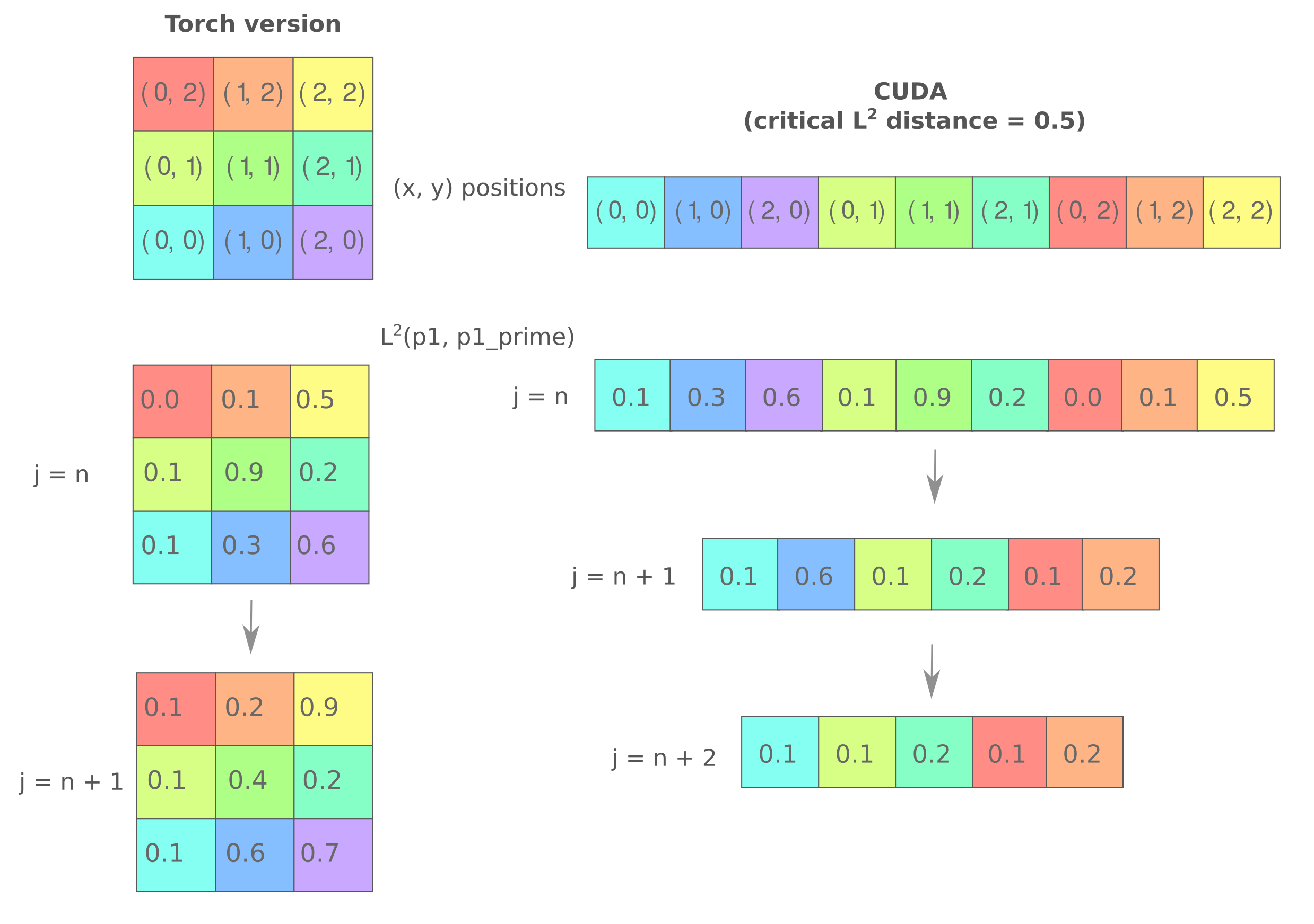
In the case of block and thread size of 1, the following depicts the difference between our early stopping CUDA code and the torch-based method employed in part 1.

With these optimizations in place, we have for a resolution of $300^2$ a runtime of

(base) bbadger@pupu:~/Desktop/threebody$ ./divergence
Elapsed Time: 44.9377s

which is a ~2.4x speedup compared to the torch code, a substantial improvement. These optimizations become more effective as the number of iterations increases (and thus the area of the input that has already diverged increases): for example, for $i=90,000$ iterations at a resolution of $1000^2$ we have a runtime of 771s for the optimized CUDA kernal but 1951s for the torch version (a 2.53x speedup) and for $i=200,000$ we have 1181s for our CUDA kernal but 4390s for the torch version (3.7x speedup). As the CUDA kernal is executed block-wise such that the computation only halts if all $i$ indicies for that block evaluate to false, decreasing the block size (and concomitantly the number of threads per block) in the kernal execution configuration can lead to modest speedups as well.

Data precision optimization

Calculations performed in 64-bit double precision floating point format are in the case of the three body problem not optimally efficient. This is because double precision floating point numbers (according to the IEEE 754 standard) reserve 11 bits for denoting the exponent, but the three body trajectories for the cases observed in Part 1 rarely fall outside the range $[-1000, 1000]$. This means that we are effectively wasting 9 bits of information with each calculation, as the bits encode information that is unused for our simulations.

Memory optimizations for GPUs go far beyond the goal of fitting our calculation into a device’s vRAM (virtual random access memory, ie global GPU memory). To give an example, suppose we wanted to use 32-bit single precision floating point data for the three body problem computations. For a $1000^2$ resolution three body divergence computation, this decreases the memory requirements to 400MB vRAM from 685MB for double precision floating point. But single precision computation is also much faster: 50k iterations require only 215s with our optimized kernal (see above), which is less than half the time (472s) required for the same number of iterations using double precision.

Thus we could make a substantial time and memory optimization by simply converting to single precision floating point data, but this comes with a problem: single precision leads to noticeable artefacts in the resulting divergence array, which are not present when performing computation using double precision. Observe in the following plot the grainy appearance of the boundary of diverging regions near the center-right (compare this to the plots using double precision above).

In effect, what we are observing is discrete behavior between adjacent pixels, which is a typical indicator of insufficient computational precision. What we want therefore is to use the unused bits in the float exponent for the mantissa. One way to do this is to define a new C++ data type using struct and convert to and from integers at each operation, but this is not

We can attempt to increase the precision of our computations while maintaining the speedups that float offers by instead converting initial values to integers before performing computations using these integers. This is known as fixed-point arithmetic, and we will use it to increase the precision of our datatype compared to the 6 or 7 decimal places of precision offered by float.

Perhaps the fastest way of performing fixed point precision calculations using CUDA is to bit shift integer type data. Bit shifting is the process of moving bits right or left in a bitwise representation of a number: for example, the integer 7 can be represented in 8-bit unsigned integer format as 00000101, and if we bit-shift thie number to the left by two then we have 00010100, which may be accomplished in C/C++ CUDA using double less-than symbols (assuming 8-bit unsigned integer format has been implemented),

int8 number = 7 << 2 // 0010100

Similarly we can bit-shift numbers to the right as well,

int8 number = 7 >> 1 // 0000001

and in both cases the bits shifted out of the 8-bit field are lost.

To use bit shifting to perform fixed point decimal arithmetic, we simply shift all numbers by the number of bits we want to use as the decimal expansion of our approximations of real numbers, in this case 26 bits (corresponding to around 8 decimal digits). The rest of the bits correspond to the whole number portions of the real numbers we are representing. The rules for performing fixed point decimal arithmetic are simple: for addition and subtraction the shift must be made to both operands, but for multplication and division the shift must be made to only the operand that we are interested in. For example, do define fractions like critical_distance = 0.5 we shift the chosen number of bits and then use integer division by and unshifted value.

#define SHIFT_AMOUNT 26
int critical_distance = (5 << SHIFT_AMOUNT) / 10; // 0.5
int m1 = 10 << SHIFT_AMOUNT; // 10

Things are more tricky when we perform multiplication or division when we care about both operands, where if we use two’s complement (see the next section) we simply multiply operands and bit shift after doing so.

Representing negative numbers is also somewhat difficult and platform-dependent, as a signed integer may be offset by some amount (such that 00000001 signifies not 1 but $-2^{8-1}+1$) or else the first bit may signify the sign, where $10000101$ might be $-7$ and $00000101$ is $7$ and is much rarer for integer representations) or may involve two’s complement, where all bits are flipped before adding 1 (-7 is now $00000101 \to 11111010 \to 11111011$ and is much more common as it does not waste any bit space).

Unfortunately, fixed point arithmetic does not particularly effective here because the process of bit shifting itself requires much more time than a normal float computation. Performing bit-shifted fixed point arithmetic requires around 70% more time for the three body problem than float arithmetic, meaning that the performance gains from switching to floats compared to double types are nearly eliminated.

Instead of changing the precision of all array elements in our simulation, we instead consider the idea that the precision of certain computations may be less important than the precision of others. If this is the case, then we can change the precision of those precision-insensitive computations to decrease the program run-time without affecting the precision of the divergence plot itself.

Some quick experimentation convinces us that most of the CUDA kernal compute time in the three body divergence simulation is taken up by the planet acceleration computations rather than the array element updates or the divergence checks themselves. When considering one term of the $a_n$ acceleration computation,

\[a_1 = \cdots -Gm_3\frac{p_1 - p_3}{\left( \sqrt{(p_{1, x} - p_{3, x})^2 + (p_{1, y} - p_{3, y})^2 + (p_{1, z} - p_{3, z})^2} \right) ^3}\]

it may be wondered whether some of the computations in the denominator need to be quite as precise as those of the numerator. This is because for each $x, y, z$ difference terms in the denominator are raised to a power of three (which necessarily reduces the accuracy after the decimal point for floating point arithmetic) and because the denominator simply scales the numerator and does not change the vector direction.

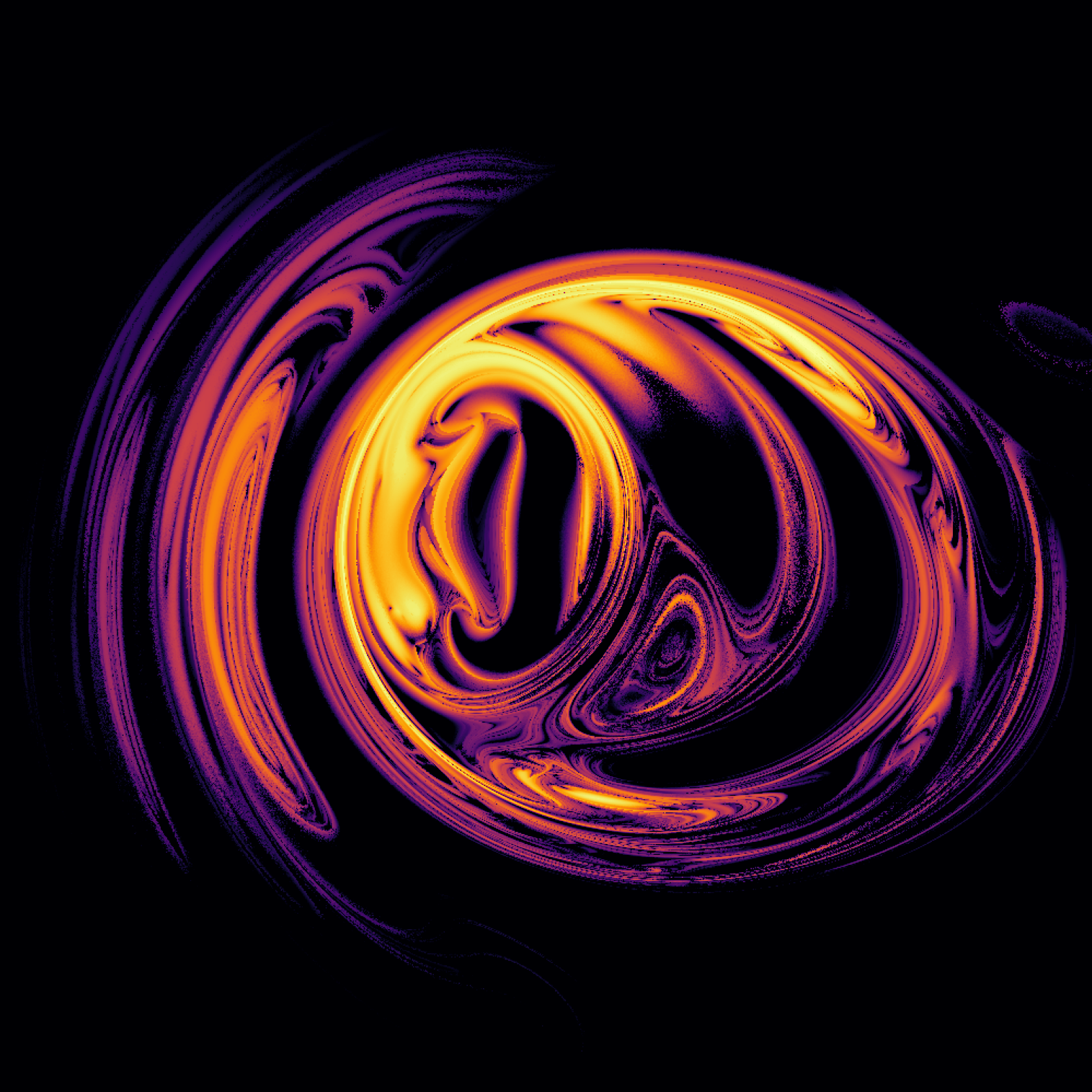
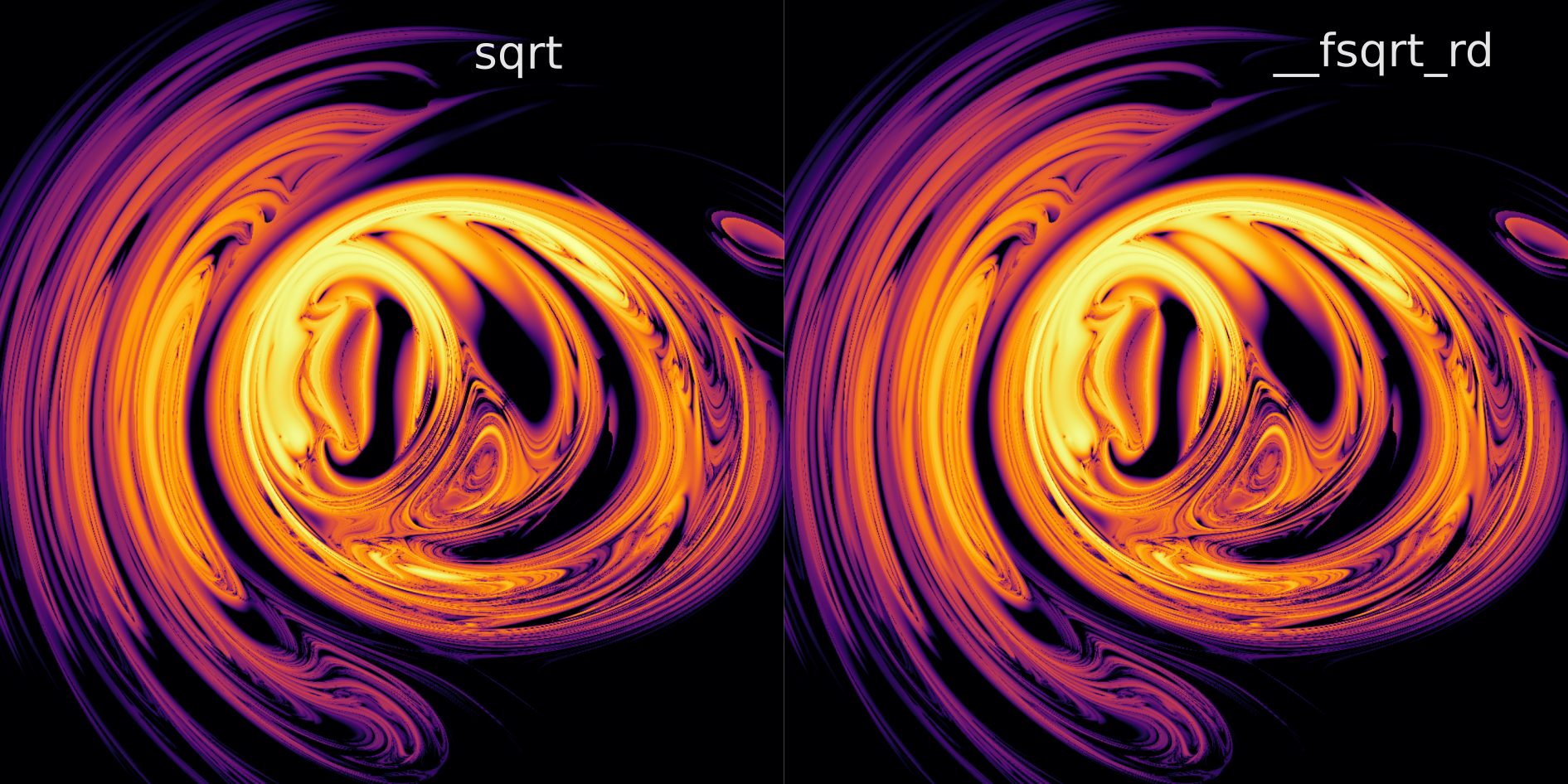
After some more experimentation we find that this guess is accurate (at least for the $x, y$ scale used previously, note that at a smaller spatial scale there is a noticeable difference in noise). Replacing each sqrt() with a single-precision (rounded down) square root function __fsqrt_rd() for $i=90,000$ iterations at a resolution of $1000^2$ we have a total runtime of 525s, which is 3.72x faster than the torch version (and 1.5x faster than the sqrt kernal). For $i=200,000$ iterations with the same resolution the fully optimized kernal requires only 851s, which is a speedup of 5.2x from the torch version. Accuracy in the divergence estimation itself is not affected, however, as the divergence plot remains identical to the double-precision square root kernal version as seen below at $i=90,000$. Thus we find that reducing the precision of the square root functions in the denominator did not change the trajectory simulations with respect to divergence (at least not at this scale), which was what we wanted.

With this much faster generation time, we can obtain larger views of the diverged regions. For a wider view of the above region, we have

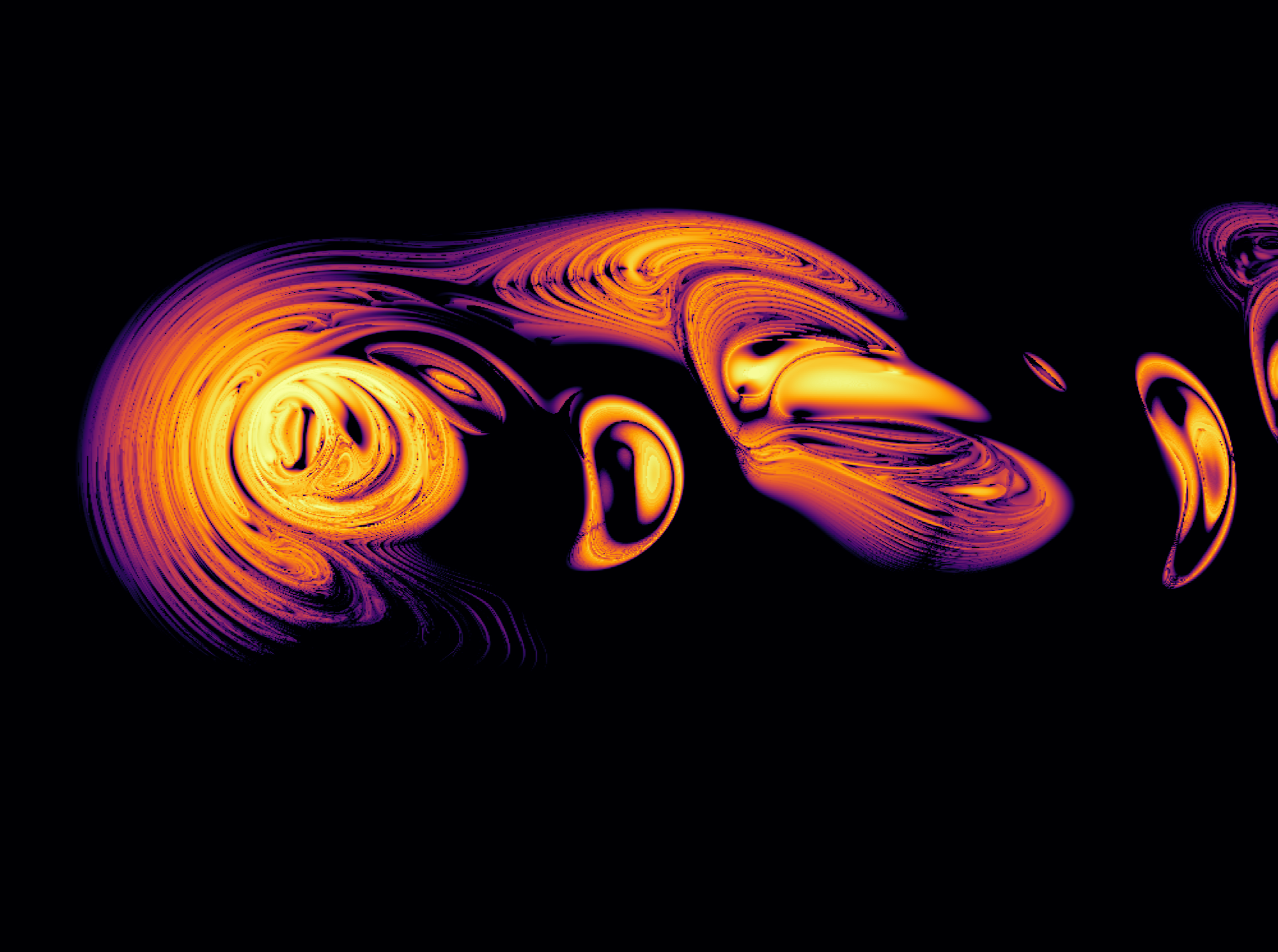
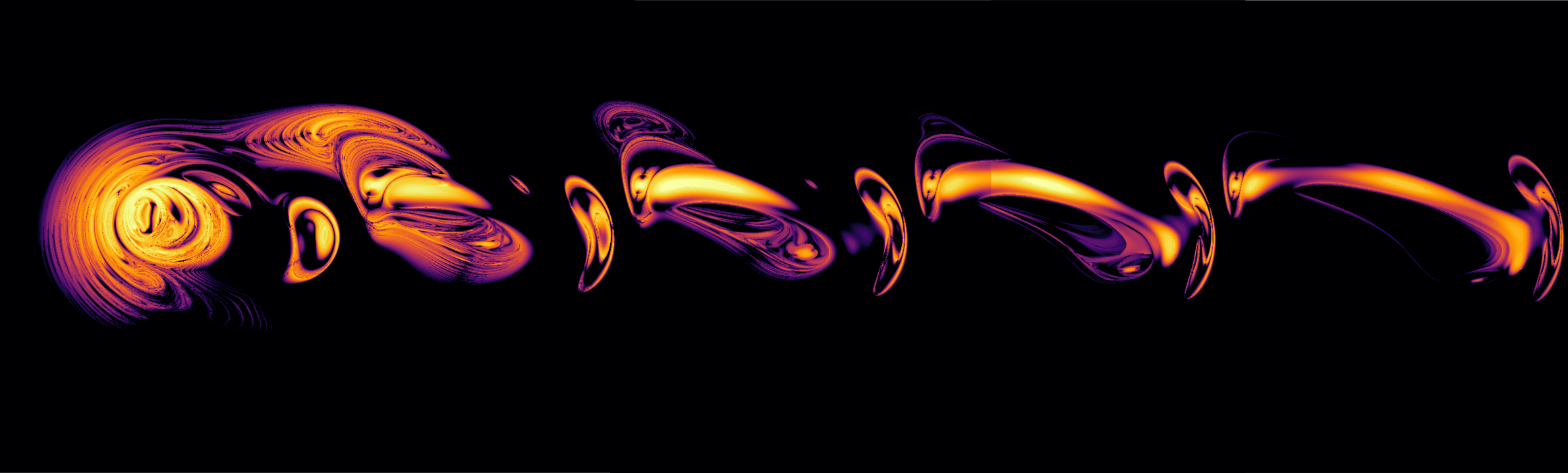
And extending the x-axis to $x \in [-40, 470]$ by stitching together multiple plots we find that the region to the right is repeated and stretched at each repetition.

Divergence fractal zoom

Thus far we have been focusing on the use of parallelized computation to map the stable (dark regions) and unstable (light regions) initial values of a planet at a familiar scale: around forty or sixty or (in the last plot) a few hundred meters. Once the divergence map is generated, can we simply find the point of interest and have an answer to whether or not that point is stable? In this section we will see that no, the question of whether a point is stable for all time is much more difficult to answer than this.

To address this question, we might want more resolution. If planet 1 at (x, y) coordinates $(-4.1, 2.3)$ diverges, what about $(-4.1001, 2.3)$? This is not possible to determine using our plot scaled at $x \in [-40, 40]$, but it may be when we compute thousands of points $x \in [-4.11, -4.10]$.

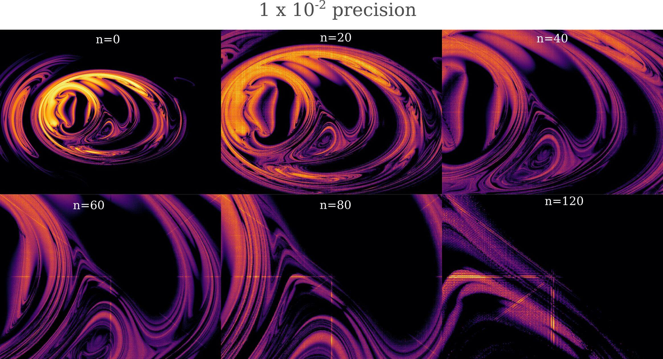
If the reader attempts to calculate these plots, they will find that there is not that much more detail present at these small scales than is found in our larger map. But it should be remembered that we seek the eventual stability or instability of these points rather than the limited approximation currently observed. In particular, for more accuracy at these smaller scales we must both increase the number of maximum iterations of our divergence plot (where each iteration is of Euler’s approximation to the solution of an ordinary differential equation, $x_{n+1} = x_n + \delta t x’_n$) as well as decrease the size of the shift performed at the start of our computation such that $x_0 - x’_0 \to 0$.

Such a zoom video becomes computationally feasible for a single GPU using the optimizations detailed in the last two sections. In the following video, the x-scale and y-scale decrease from 1.28km to 518nm, which to put in perspective means that each pixel is separated from its neighbors by the width of an atom.

This video demonstrates a manifestation of why the three body problem is unsolvable: extreme sensitivity to initial conditions. Here we see that at scales down to the width of an atom, stable and unstable trajectories may be arbitrarily close to one another. It is not hard to see that this phenomenon is by no means limited to the scales we have investigated here but extends towards the infinitely small. Indeed, sensitivity to initial conditions stipulates that for any point in our x, y grid any other point arbitrarily close will eventually diverge, but difference in relative stability will also tend to infinity as $t \to \infty$ and $x_0 - x’_0 \to 0$.

This method is straightforward to implement but results in an increase in the amount of computation required for each successively smaller field of view. Practically speaking this means that even with the optimized CUDA kernal, it takes days to finish the computations required for a zoom video from the tens of meters range (in $x, y$) down to the micrometer range. A little experimentation shows us that subsituting the single-precision square root operation for the double-precision is no longer sufficient around the millimeter scale, as noise begins to overwhelm the divergence plot patterns if this substitution is made.

How can we reduce the amount of computation per frame in a video on divergence? In other words, given a sequence of divergence maps of decreasing domain sizes, centered on the same region, can we reduce the amount of computation required for some or all of these maps? One way to reduce the total computation amount is to attempt to re-use previously computed values: if the divergence values for $(x, y)$ coordinates calcuated at one scale are again needed at a smaller scale, we can simply save that divergence value and look it up rather than re-calculating.

To implement this cached zoom approach, we can either save values in a cache in C++ such that the cache memory is not freed each time the kernal is called or else we can have the cache in the Python code that uses ctypes to interface with our .so CUDA kernal. Here we will explore the latter, although there is no real expected performance difference between these approaches.

Therefore we start by initializing our already_computed cache as a Python dictionary

# python
already_computed = {}

and then we initialize the time_steps and shift_distance variables such that the number of timesteps increases linearly while the shifted distance decreases logarithmically as the zoom video frame number increases. Likewise we can specify the rate at which we are zooming in on the point x_center, y_center by dividing our initial range by the power of two appropriate. In the code below, dividing the video iteration i by 30 serves to have the video halve in range for every 30 frames.

Another decision to be made is how we want to look up coordinates that are sufficiently close to previously computed coordinates. For simplicity we will just round to a decimal place denoted by the variable decimal, which needs to increase as the scale decreases to maintain resolution.

last_time_steps = 0
video_frames = 500
for i in range(video_frames):
	x_res, y_res = 1000, 1000
	...
	x_range = 40 / (2**(i/30))
	decimal = int(-np.log(x_range / (x_res)))

Before looking up the values, we need to increment the number of expected iterations until divergence for each stored input (because the number of iterations is continually increasing as the range decreases).

	for pair in already_computed:
		already_computed[pair] += time_steps - last_time_steps
	last_time_steps = time_steps

Now we assemble an array of all locations that we do not have a stored value for,

	start_x = x_center - x_range/2
	start_y = y_center - y_range/2
	for j in range(int(x_res*y_res)):
		remainder = j % y_res
		step = j // x_res
		x_i = start_x + x_range*(remainder/x_res)
		y_i = start_y + y_range*(step/y_res)

		if (round(x_i, decimal), round(y_i, decimal)) not in already_computed:
			x.append(x_i) 
			y.append(y_i)
			return_template.append(-1)
		else:
			return_template.append(already_computed[(round(x_i, decimal), round(y_i, decimal))])
	length_x, length_y = len(x), len(y)

and next we need to modifying the CUDA kernal driver C++ function to accept array objects (pointers) x, y.

	f = ctypes.CDLL('./divergence_zoom.so').divergence
	x_array_type = ctypes.c_float * len(x)
	y_array_type = ctypes.c_float * len(y)
	x = x_array_type(*x)
	y = y_array_type(*y)

	f.argtypes = [ctypes.c_int, 
		ctypes.c_int, 
		ctypes.c_int, 
		ctypes.c_double, 
		ctypes.c_double, 
		ctypes.c_double, 
		ctypes.c_double, 
		ctypes.c_double, 
		ctypes.POINTER(ctypes.c_float*len(x)), 
		ctypes.POINTER(ctypes.c_float*len(y)),
		ctypes.c_int
		] 

	f.restype = ctypes.POINTER(ctypes.c_int * length_x) # kernal return type
	arr = f(x_res, y_res, time_steps, x_center, x_range, y_center, y_range, shift_distance, x, y, length_x).contents
	time_array = np.array(arr)
	flattened_arr = time_array.flatten()
	return_arr = []
	inc = 0
	for k in range(len(return_template)):
		if return_template[k] == -1:
			return_arr.append(flattened_arr[inc])
			already_computed[(round(x[inc], decimal), round(y[inc], decimal))] = flattened_arr[inc]
			inc += 1
		else:
			return_arr.append(return_template[k])
	output_array = np.array(return_arr).reshape(x_res, y_res)
	output_array = time_steps - output_array
	plot(output_array, i)

Deleting cache keys that are out-of-range or with too small precision allows us to prevent the cache from growing too large as the zoom video is computed.

Unfortunately, when implemented we see that this method has a significant flaw: we don’t really want to re-use precomputed divergence computations from larger scales at smaller even if they are incremented to match an expected value for more total iteration. Because of sensitivity to initial conditions, such incremented estimates are bound to become more inaccurate the larger the difference in scale (and thus the number of maximum iterations). Our method of saving the values of certain elements is useful only if we can recall the values of elements at much smaller elements.

For example, observe the following figure where the decimal precision is fixed (and so the time to compute each successive iteration heads to zero as the zoom iteration increases).

Multistep Linear Methods

It is a not generally well-known fact that although the advances in computational speed due to hardware and software have led to speed decreases on the order ot $10^7$ over the last seventy years, the advances in terms of better algorithms for many problems in the field of numerical analysis (which this work may be thought to fall under) during this same time have led to speed decreases that exceed even that of rapidly advancing hardware.

When we consider the three body problem divergence plot computation from an algorithmic optimization perspective, one apparent place for such optimization is in the number of iterations required for the plot which is generally on the order of $50,000$ but increases to more than $500,000$ at small scales. So far we have optimized the computations per time step and removed superfluous steps for diverged trajectories but we have not

The special case of a multistep linear method with only one step is just Euler’s method.

\[x_{n+1} = x_n + \Delta t * f(x_n)\]

For the three body problem we must adapt this method somewhat as we can only compute acceleration using three variables (ie for the three body problem, positions of $x, y z$), but we cannot apply acceleration directly to position. Instead we calculate the velocity $v$ from acceleration $v’$ before finding the next position $p_{n+1}$ from $p_{n}$ as follows:

\[v(x, y, z)_{n+1} = v(x, y, z)_n + \Delta t * v' ((x, y, z)_n) \\ p(x, y, z)_{n+1} = p(x, y, z)_n + \Delta t * v((x, y, z)_n)\]

To increase the order of the convergence of this dynamical system, we may use a higher-order linear multistep method, also known as Adams-Bashforth methods. The order of convergence is determined by the number of terms the method has, for example the two-step method

\[x_{n+2} = x_n + \Delta t * \frac{1}{2}(3 f(x_{n+1}) - 1f(x_n))\]

converges quadratically, and the four-step method

\[x_{n+4} = x_n + \Delta t * \frac{1}{24}(55f(x_{n+3}) - 59f(x_{n+2}) + 37f(x_{n+1}) - 9f(x_n))\]

converges with order 4. There are some choices available to us for how these methods are adapted to the three body problem trajectories, and below is an example of using a second-order multistep method for both velocity and position computation.

\[v(x, y, z)_{n+2} = v(x, y, z)_n + \Delta t * \frac{1}{2}(3v' ((x, y, z)_{n+1}) - 1v'((x, y, z)_n)\\ p(x, y, z)_{n+2} = p(x, y, z)_n + \Delta t * \frac{1}{2}(3v ((x, y, z)_{n+1}) - 1v((x, y, z)_n)\]

It may be unclear how one is supposed to first find $x_{n+1}, x_{n+2}…$ given only $x_n$ while using an order >1 multistep method. Here we use a one-step (Euler’s) method for computing the first $x_{n+1}$.

Because multistep methods converge faster than the one-step Euler’s method, we can in principle take fewer steps at a larger step size while maintaining accuracy. The computational requirements for the three body problem scale somewhat less than linearly with the number of steps required, so reducing a step number by a factor of 10 leads to a substantial speedup.

The order 4 linear multistep method may be implemented using a queue as follows:

def adams_bashforth(self, current, fn_arr):
	assert len(fn_arr) >= order

	# note that array is newest to the right, oldest left
	fn, fn_1, fn_2, fn_3 = fn_arr[-1], fn_arr[-2], fn_arr[-3], fn_arr[-4]
	v = current + (1/24) * self.delta_t * (55*fn - 59*fn_1 + 37*fn_2 - 9*fn_3)
	return v

where for each array we compute and pop the oldest computed fn value, for example the velocity computation is as follows:

dv1_arr = deque([])
...
nv1 = self.adams_bashforth(self.v1, dv1_arr)
dv1_arr.popleft()

When we apply linear multistep method to three body problem trajectories, we see that indeed the use of second or fourth-order updates allows for the use of a larger step size

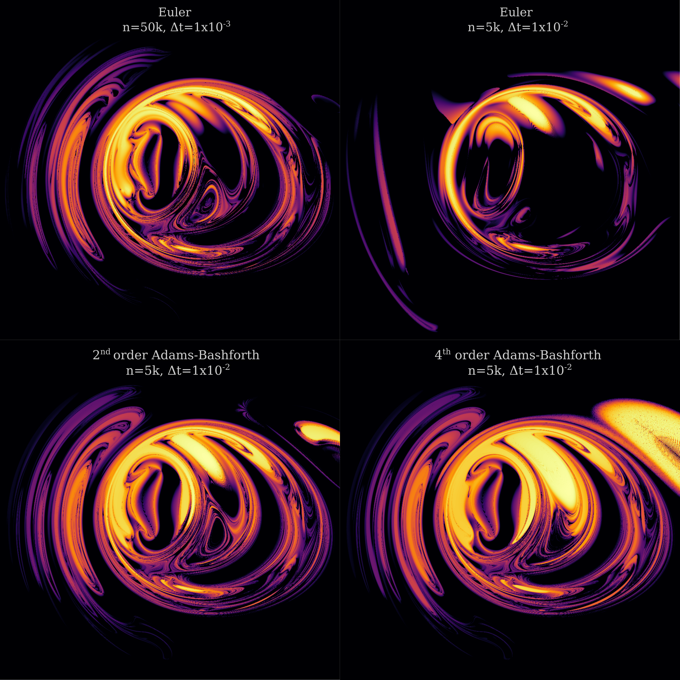
There is a problem with this approach, however: at very small scales, the use of a larger step size results in numerical artefacts regardless of the method used. For example, we can see vertical lines of quickly-diverging regions appear for Euler’s method as well as order 2 or order 4 Adams-Bashforth methods, which are absent from the order 1 method (Euler’s).

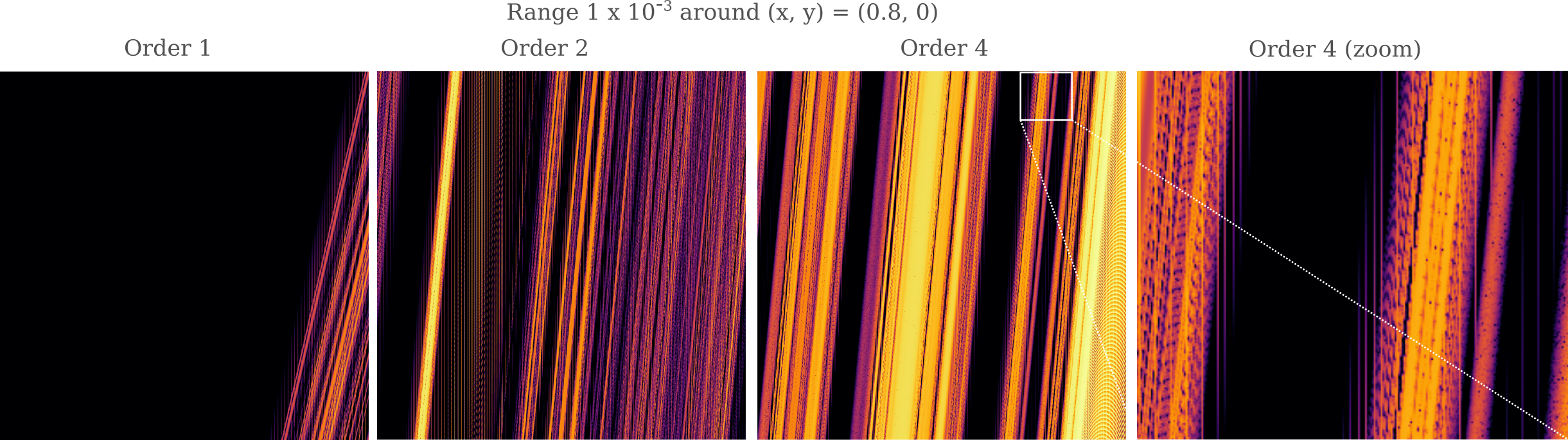
These are evidently numerical instabilities in the calculation of the three body divergence, which leads to discrete shifts in stability for adjacent pixels (which is not expected to occur for our simulation unless the number of time steps heads towards infinity and the initial shift heads towards zero). These instabilities lead to repetitive shifts in stability, where alternating patterns of stable and unstable regions exist.