The three body problem

Newtonian mechanics

Newtonian mechanics are often thought to render the motion of planets and stars a solved problem: as the laws of motion have been found, the only thing left to do is to apply them to the heavenly bodies to know where they will go. Consulting the section on Newtonian mechanics in Feynman’s lectures on physics (vol. 1 section 9-9), we find this confident statement:

“Now armed with the tremendous power of Newton’s laws, we can not only calculate such simple motions but also, given only a machine to handle the arithmetic, even the tremendously complex motions of the planets, to as high a degree of precision as we wish!”

This statement seems logical at first glance, and was the hope of Laplace and others immediately following Newton (but not, as we shall see, of Feynman). The most accurate equations of force, momentum, and gravitational acceleration are all fairly simple and for most examples that are taught in school, there are solutions that do not involve time at all. We can define the differential equations for which there exists a closed (non-infinite, or in other words practical) solution that does not contain any reference to the variable time as ‘solved’. The mechanics most of us learned were problems that were solvable with some calculus, usually by integrating over time to remove that variable. The solution furthermore must be of finite length, and cannot itself grow as time increases.

If one peruses the curriculum generally taught to people just learning mechanics, a keen eye might spot something curious: the systems considered in the curriculum are all systems of two objects: a planet and a moon, or else the sun and earth. This is the problem Newton inherited from Kepler, and the solution he found is the one we learn about today.

But what about 3 bodies, or more? Newton attempted to find a similar solution to this problem but failed. This did not deter others, and it seems that some investigators (Laplace in particular) were confident of a solution being just around the corner, even if they could not find one themselves.

The three body problem may be formulated as follows:

\[a_1 = -Gm_2\frac{p_1 - p_2}{\lvert p_1 - p_2 \rvert ^3} - Gm_3\frac{p_1 - p_3}{\lvert p_1 - p_3 \rvert^3} \\ \; \\ \; \\ a_2 = -Gm_3\frac{p_2 - p_3}{\lvert p_2 - p_3 \rvert ^3} - Gm_1\frac{p_2 - p_1}{\lvert p_2 - p_1 \rvert^3} \\ \; \\ \; \\ a_3 = -Gm_1\frac{p_3 - p_1}{\lvert p_3 - p_1 \rvert ^3} - Gm_2\frac{p_3 - p_2}{\lvert p_3 - p_2 \rvert^3}\]

where $p_i = (x_i, y_i, z_i)$ and $a_i$ refers to the acceleration of $p_i$, ie

\[a_i = (\ddot x_i, \ddot y_i, \ddot z_i)\]

Note that $\lvert p_1 \rvert$ signifies a vector norm, not absolute value or cardinality. The vector norm is the distance to the origin, calculated in three dimensions as

\[\lvert p_1 \rvert = \sqrt {x_1^2 + y_1^2 + z_1^2}\]

The norm of the difference of two vectors may be understood as a distance between those vectors, if our distance function is an arbitrary dimension -extension of the function above.

Modeling the three body problem

After a long succession of fruitless attempts, Bruns and Poincare showed that the three body problem does not contain a solution approachable with the method of integration used by Newton to solve the two body problem. No one could solve the three body problem, that is, make it into a self-contained algebraic expression, because it is impossible to do so!

Is any solution possible? Sundman found that there is an infinite power series that describes the three body problem, and in that sense there is. But in the sense of actually predicting an orbit, the power series is no help because it cannot directly infer the position of any of the three bodies owing to round-off error propegation from extremely slow convergence (ref). From the point of a solution being one in which time is removed from the equation, the power series is more of a problem reformulation than a solution: the time variable is the power series base. Rather than numerically integrate the differential equations of motion, one can instead add up the power series terms, but the latter option takes an extremely long time to do. To give an appreciation for exactly how long, it has been estimated that more than $10^{8000000}$ terms are required for calculating the series for one short time step (ref).

For more information, see Wolfram’s notes.

Unfortunately for us, there is no general solution to the three body problem: we cannot actually tell where three bodies will be at an arbitrary time point in the future, let alone four or five bodies. This is an inversion with respect to what is stated in the quotation above: armed with the power of Newton’s laws, we cannot calculate, with arbitrary precision in finite time, the paths of any system of more than two objects.

Bounded trajectories of 3 objects are almost always aperiodic

Why is there a solution to the two body problem but not three body problem? One can imagine that a problem with thousands of objects would be much harder to deal with than two objects, but why does adding only one more object create such a difficult problem?

One way to gain an appreciation for why is to simply plot some trajectories. Let’s do this using python. To start with, a docstring is added and the relevant libraries are imported.

#! python3
# A program that produces trajectories of three bodies
# according to Netwon's laws of gravitation

# import third-party libraries
import numpy as np 
import matplotlib.pyplot as plt 
from mpl_toolkits.mplot3d import Axes3D
plt.style.use('dark_background')

Next we can specify the initial conditions for our three bodies. Here we have bodies with masses of 10, 20, and 30 kilograms, which could perhaps be a few small asteroids orbiting each other. We then specify their initial positions and velocities, and for simplicity we assume that the bodies are very small such that collisions do not occur.

# masses of planets
m_1 = 10
m_2 = 20
m_3 = 30

# starting coordinates for planets
# p1_start = x_1, y_1, z_1
p1_start = np.array([-10, 10, -11])
v1_start = np.array([-3, 0, 0])

# p2_start = x_2, y_2, z_2
p2_start = np.array([0, 0, 0])
v2_start = np.array([0, 0, 0])

# p3_start = x_3, y_3, z_3
p3_start = np.array([10, 10, 12])
v3_start = np.array([3, 0, 0])

Now for a function that calculates the change in velocity (acceleration) for each body, referred to as planet_1_dv etc. that uses the three body formulas above.

def accelerations(p1, p2, p3):
	"""
	A function to calculate the derivatives of x, y, and z
	given 3 object and their locations according to Newton's laws
	
	"""

	m_1, m_2, m_3 = self.m1, self.m2, self.m3
	planet_1_dv = -9.8 * m_2 * (p1 - p2)/(np.sqrt((p1[0] - p2[0])**2 + (p1[1] - p2[1])**2 + (p1[2] - p2[2])**2)**3) - \
		       9.8 * m_3 * (p1 - p3)/(np.sqrt((p1[0] - p3[0])**2 + (p1[1] - p3[1])**2 + (p1[2] - p3[2])**2)**3)

	planet_2_dv = -9.8 * m_3 * (p2 - p3)/(np.sqrt((p2[0] - p3[0])**2 + (p2[1] - p3[1])**2 + (p2[2] - p3[2])**2)**3) - \
		       9.8 * m_1 * (p2 - p1)/(np.sqrt((p2[0] - p1[0])**2 + (p2[1] - p1[1])**2 + (p2[2] - p1[2])**2)**3)

	planet_3_dv = -9.8 * m_1 * (p3 - p1)/(np.sqrt((p3[0] - p1[0])**2 + (p3[1] - p1[1])**2 + (p3[2] - p1[2])**2)**3) - \
		       9.8 * m_2 * (p3 - p2)/(np.sqrt((p3[0] - p2[0])**2 + (p3[1] - p2[1])**2 + (p3[2] - p2[2])**2)**3)

	return planet_1_dv, planet_2_dv, planet_3_dv
	

A time step size delta_t is chosen, which should be small for accuracy, and the number of steps are specified and an array corresponding to the trajectory of each point is initialized. Varying initial velocites are allowed, so both position and velocity require array initialization.

# parameters
delta_t = 0.001
steps = 200000

# initialize trajectory array
p1 = np.array([[0.,0.,0.] for i in range(steps)])
v1 = np.array([[0.,0.,0.] for i in range(steps)])

p2 = np.array([[0.,0.,0.] for j in range(steps)])
v2 = np.array([[0.,0.,0.] for j in range(steps)])

p3 = np.array([[0.,0.,0.] for k in range(steps)])
v3 = np.array([[0.,0.,0.] for k in range(steps)])

The first element of each position and velocity array is assigned to the variables denoting starting coordinates,

# starting point and velocity
p1[0], p2[0], p3[0] = p1_start, p2_start, p3_start

v1[0], v2[0], v3[0] = v1_start, v2_start, v3_start

and the velocity and position at each point is calculated for each time step. For clarity, a two-step approach is chosen here such that the three body eqution is used to calculate the accelerations for each body given its position. Then the acceleration is applied using Euler’s method such that a new velocity v1[i + 1] is calculated. Using the current velocity, the new position p1[i + 1] is calculated using Euler’s formula.

# evolution of the system
for i in range(steps-1):
	# calculate derivatives
	dv1, dv2, dv3 = accelerations(p1[i], p2[i], p3[i])

	v1[i + 1] = v1[i] + dv1 * delta_t
	v2[i + 1] = v2[i] + dv2 * delta_t
	v3[i + 1] = v3[i] + dv3 * delta_t

	p1[i + 1] = p1[i] + v1[i] * delta_t
	p2[i + 1] = p2[i] + v2[i] * delta_t
	p3[i + 1] = p3[i] + v3[i] * delta_t

After the loop above runs, we are left with six arrays: three position arrays and three velocity arrays containing information on each body at each time step. For plotting trajectories, we are only interested in the position at each time. Some quick list comprehension can separate x, y, and z from each array for the plt.plot() method. p1, p2, and p3 are colored red, white, and blue, respectively.

fig = plt.figure(figsize=(8, 8))
ax = fig.gca(projection='3d')
plt.gca().patch.set_facecolor('black')

plt.plot([i[0] for i in p1], [j[1] for j in p1], [k[2] for k in p1] , '^', color='red', lw = 0.05, markersize = 0.01, alpha=0.5)
plt.plot([i[0] for i in p2], [j[1] for j in p2], [k[2] for k in p2] , '^', color='white', lw = 0.05, markersize = 0.01, alpha=0.5)
plt.plot([i[0] for i in p3], [j[1] for j in p3], [k[2] for k in p3] , '^', color='blue', lw = 0.05, markersize = 0.01, alpha=0.5)

plt.axis('on')

# optional: use if reference axes skeleton is desired,
# ie plt.axis is set to 'on'
ax.set_xticks([]), ax.set_yticks([]), ax.set_zticks([])

# make panes have the same color as the background
ax.w_xaxis.set_pane_color((0.0, 0.0, 0.0, 1.0)), ax.w_yaxis.set_pane_color((0.0, 0.0, 0.0, 1.0)), ax.w_zaxis.set_pane_color((0.0, 0.0, 0.0, 1.0))
plt.show()
plt.close()

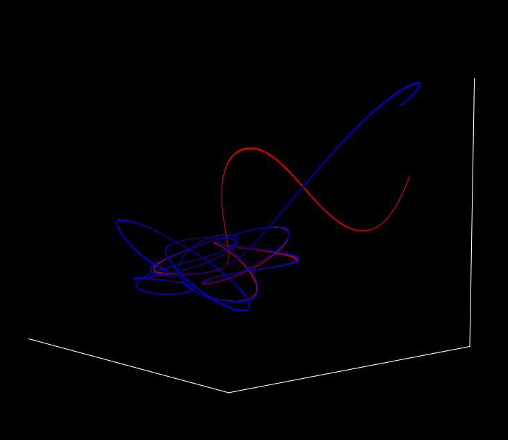
And we are done! This yields the following map of the trajectories in 3D space.

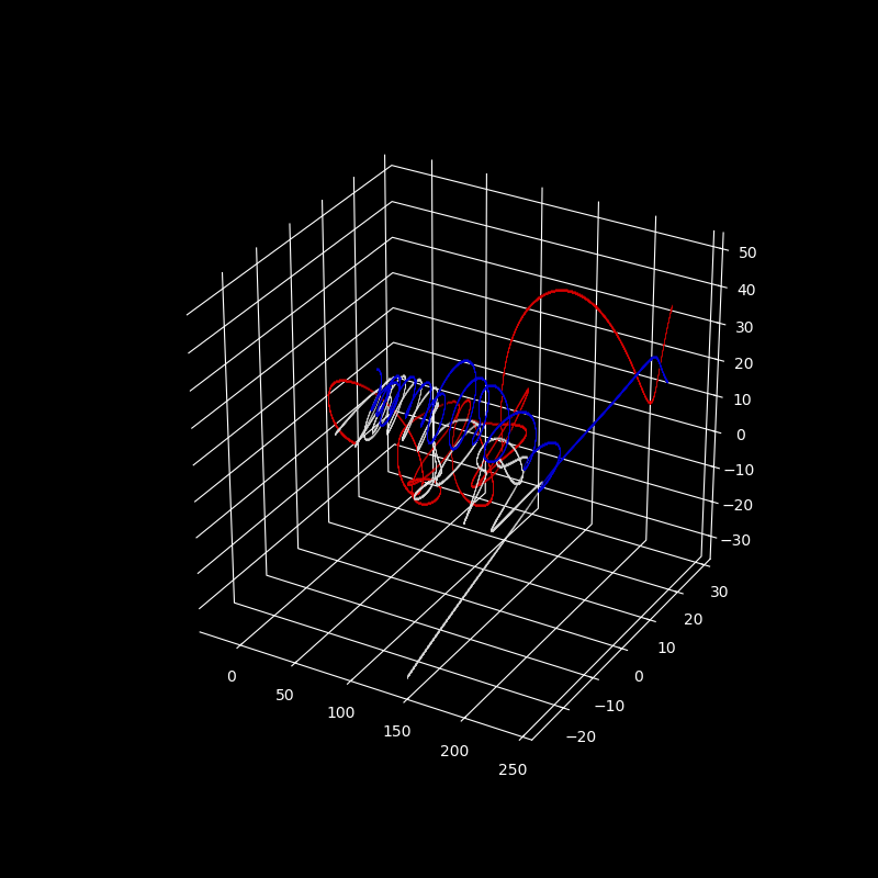
With grid lines removed for clarity (ax.set_xticks([]), ax.set_yticks([]), ax.set_zticks([]) removed),

The orientation of the view can be specified using the interactive matplotlib interface if plt.show() is called, and if images are saved directly then plt.view_init() should be used as follows:

...
ax.view_init(elev = 10, azim = 40)
plt.savefig('{}'.format(3_body_image), dpi=300)

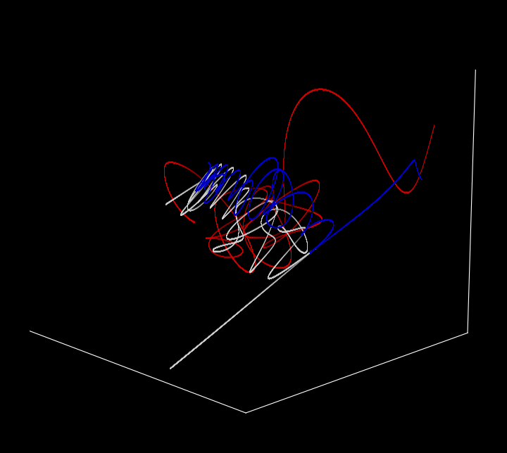
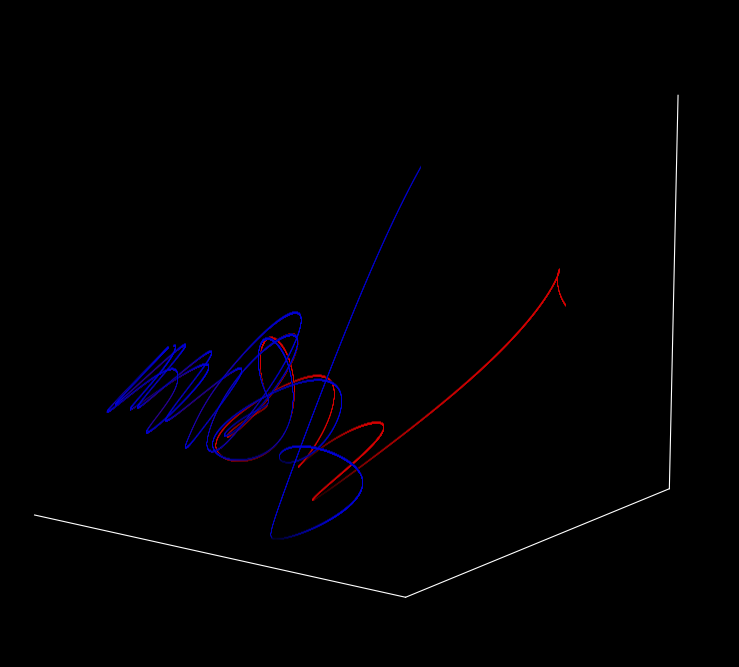
Over time (sped up for brevity) and from a slightly different perspective, the trajectory is

Poincaré and sensitivity to initial conditions

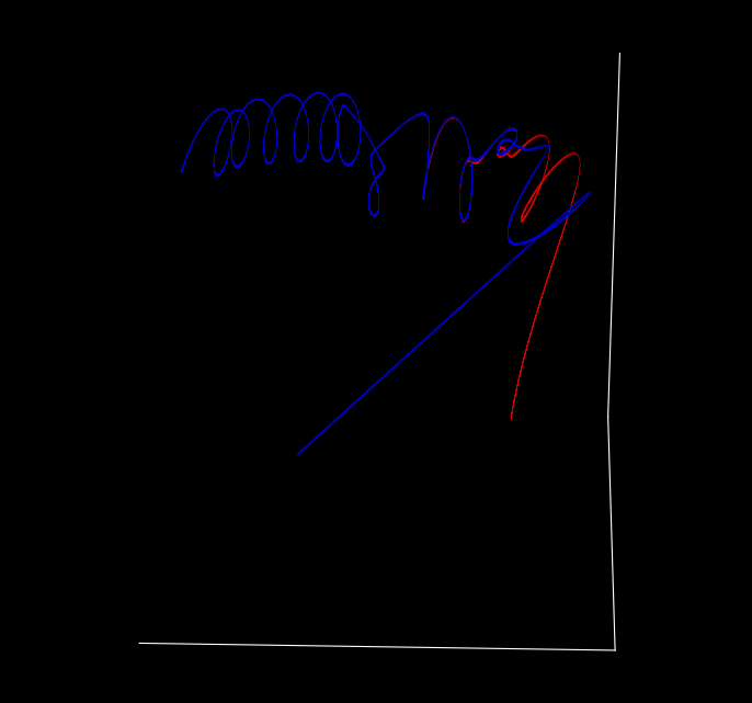
What happens when we shift the starting position of one of the bodies by a miniscule amount? Changing the z position of the third body from $12$ to $12.000001$ yields

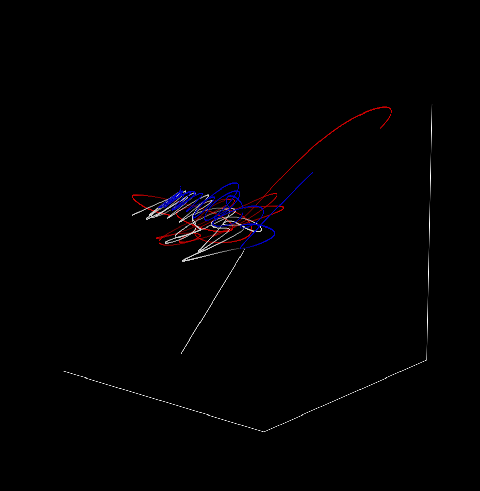
The trajectories are different to what was observed before, but how so? The new image has different x, y, and z-scales than before and individual trajectories are somewhat difficult to make out.

If we compare the trajectory of the first body to it’s trajectory (here red) in the slightly shifted scenario (blue),

from the side and over time, we can see that they are precisely aligned for a time but then diverge, first slowly then quickly.

The same is true of the second body (red for original trajectory, blue for the trajectory when the tiny shift to the third body’s initial position has been made)

And of the third as well.

Plotting the distance between each point and its counterpart as follows

distance_2 = []
for i in range(steps):
	distance_2.append(np.sqrt(np.sum([j**2 for j in p2[i] - p2_prime[i]])))

distance_1 = []
for i in range(steps):
	distance_1.append(np.sqrt(np.sum([j**2 for j in p1[i] - p1_prime[i]])))

distance_3 = []
for i in range(steps):
	distance_3.append(np.sqrt(np.sum([j**2 for j in p3[i] - p3_prime[i]])))

fig, ax = plt.subplots()
ax.plot(time, distance_1, alpha=0.5, color='red')
ax.plot(time, distance_2, alpha=0.5, color='grey')
ax.plot(time, distance_3, alpha=0.5, color='blue')
plt.ylim(0, 120)
ax.set(xlabel='time', ylabel='Distance')
plt.show()
plt.close()

yields

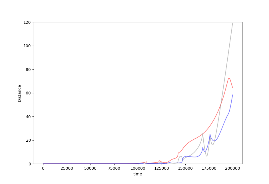
In 1914, H. Poincaré observed that “small differences in initial conditions produce very great ones in the final phenomena” (as quoted here).

If we make slightly worse and worse initial measurements, does the inaccuracy of our prediction get worse too? Surprisingly the answer to this question is often but not always. To see how, here we iterate the distance measurement above but change the distance between planet 3 and its ‘true’ value to increase from $\Delta z = 0.00000001 \to \Delta z = 0.00001$

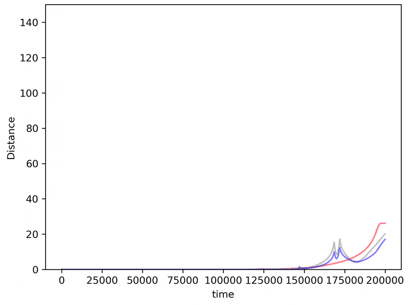
Just as for the logistic map, the benefit we achieve for getting better initial accuracies is unpredictable. Sometimes a better initial measurement will lead to larger errors in prediction!

Divergence and Smale Horseshoes with Homoclinic Tangles

We have so far observed the behavior of only one initial set of points in three-dimensional space for each planet. But it is especially interesting to consider the behavior of many initial points. One could consider the behavior of all points in $\Bbb R^3$, but this is often difficult to visualize as the trajectories may form something like a solid object. To avoid this difficulty, we can restrict our initial points to some subspace.

In $\Bbb R^3$ we can choose vectors in two basis vectors, perhaps $x, y$, to vary while the third $z$ stays constant. Allowing two basis vectors to change freely in $\Bbb R^3$ forms a two-dimensional sheet in that three-dimensional space, or in other words forms a plane. What happens to points embedded in this plane as they observe Newton’s laws of gravitation, and in particular do different points in this plane have different sensitivities to initial conditions? Another way of saying this is that we will ask the question of which starting positions diverge earlier, and which diverge later.

As we have three bodies, we can choose one of these (say p1) to allow to start in different locations in a two-dimensional plane while holding the other two bodies fixed in their starting points before observing the trajectory resulting from each of these different starting locations. As we are interested in divergence, we can once again compare the trajectory of the planet p1 at each of these starting points to a slightly shifted planet p1_prime. As we are now dealing with an multidimensional array of initial points rather than only three per planet, a slightly different approach is required. Code snippets and the overall approach will be described here, and the complete program may be found in this source code file.

Our computational structure to calculate sensitivity is initialized by changing the 3x1x1 initial point for planet 1 to an array of size 3 byy_res by x_res for that planet. For example, if we want to plot 100 points along both the x and y-axis we start with a 3x1000x1000 size array for p1.

def sensitivity(self, y_res, x_res, steps, double_type=True):
	"""
	Plots the sensitivity to initial values per starting point of planet 1, as
	measured by the time until divergence.
	"""

	delta_t = self.delta_t
	y, x = np.arange(-20, 20, 40/y_res), np.arange(-20, 20, 40/x_res)
	grid = np.meshgrid(x, y)
	grid2 = np.meshgrid(x, y)

	# grid of all -11, identical starting z-values
	z = np.zeros(grid[0].shape) - 11

	# shift the grid by a small amount
	grid2 = grid2[0] + 1e-3, grid2[1] + 1e-3
	# grid of all -11, identical starting z-values
	z_prime = np.zeros(grid[0].shape) - 11 + 1e-3

	# p1_start = x_1, y_1, z_1
	p1 = np.array([grid[0], grid[1], z])
	p1_prime = np.array([grid2[0], grid2[1], z_prime])
		

But now we also have to have arrays of identical dimensions for all the other planets, as their trajectories each depend on the initial points of planet 1. This means that we must make arrays that track the motion of each planet in three-dimensional space for all points in the initial plane of possible planet 1 values.

For example, planet two can be initialized to the same value as in our approach above, or $(0, 0, 0)$ for both position and velocity, with the following:

	p2 = np.array([np.zeros(grid[0].shape), np.zeros(grid[0].shape), np.zeros(grid[0].shape)])
	v2 = np.array([np.zeros(grid[0].shape), np.zeros(grid[0].shape), np.zeros(grid[0].shape)])
	...

Numpy is an indespensible library for mathematical computations, but there are others that may be faster for certain computations. To speed up the three body divergence calculations we can employ pytorch to convert these numerical arrays from numpy.ndarray() objects to torch.Tensor() as follows:

	# convert numpy arrays to torch.Tensor() objects (2x speedup with cpu)
	p1, p2, p3 = torch.Tensor(p1), torch.Tensor(p2), torch.Tensor(p3)
	...

before doing the same for v1, v2, v3, p1_prime, etc. If the device performing these computations contains a graphics processing unit, these arrays can be computed using that by specifying p1 = torch.Tensor(p1, device=torch.device('cuda')) for each torch.Tensor() object to speed up the computations even further.

Sensitivity to initial values can be tested by observing if any of the p1 trajectories have separated significantly from the shifted p1_prime values. This is known as divergence, and the following function creates a boolean array to see which points have separated (diverged):

def not_diverged(self, p1, p1_prime):
	"""
	Find which trajectories have diverged from their shifted values

	Args:
		p1: np.ndarray[np.meshgrid[bool]]
		p1_prime: np.ndarray[np.meshgrid[bool]]

	Return:
		bool_arr: np.ndarray[bool]

	"""
	separation_arr = np.sqrt((p1[0] - p1_prime[0])**2 + (p1[1] - p1_prime[1])**2 + (p1[2] - p1_prime[2])**2)
	bool_arr = separation_arr <= self.distance
	return bool_arr
		

Using this function to test whether or not planet 1 has diverged from its shifted planet 1 prime,

def sensitivity(self, y_res, x_res, steps, double_type=True):
	...
	time_array = np.zeros(grid[0].shape)
	# bool array of all True
	still_together = grid[0] < 1e10
	t = time.time()

	# evolution of the system
	for i in range(self.time_steps):
		if i % 100 == 0:
			print (i)
			print (f'Elapsed time: {time.time() - t} seconds')

		not_diverged = self.not_diverged(p1, p1_prime)
		# convert Tensor[bool] object to numpy array
		not_diverged = not_diverged.numpy()
		
		# points still together are not diverging now and have not previously
		still_together &= not_diverged

		# apply boolean mask to ndarray time_array
		time_array[still_together] += 1

now we can follow the trajectories of each planet at each initial point. Note that these trajectories are no longer tracked, as doing so requires an enormous amount of memory. Instead the points and velocities are simply updated at each time step.

		# calculate derivatives
		dv1, dv2, dv3 = self.accelerations(p1, p2, p3)
		dv1_prime, dv2_prime, dv3_prime = self.accelerations(p1_prime, p2_prime, p3_prime)

		nv1 = v1 + dv1 * delta_t
		nv2 = v2 + dv2 * delta_t
		nv3 = v3 + dv3 * delta_t

		p1 = p1 + v1 * delta_t
		p2 = p2 + v2 * delta_t
		p3 = p3 + v3 * delta_t
		v1, v2, v3 = nv1, nv2, nv3

After $50,000$ time steps, initial points on the $x, y$ plane of planet 1 (y-axis running top to bottom and x-axis running left to right) on both x- and y-axes such that the top left is $(y, x) = (-20, -20)$ and the bottom right is $(y, x) = (20, 20)$) we have

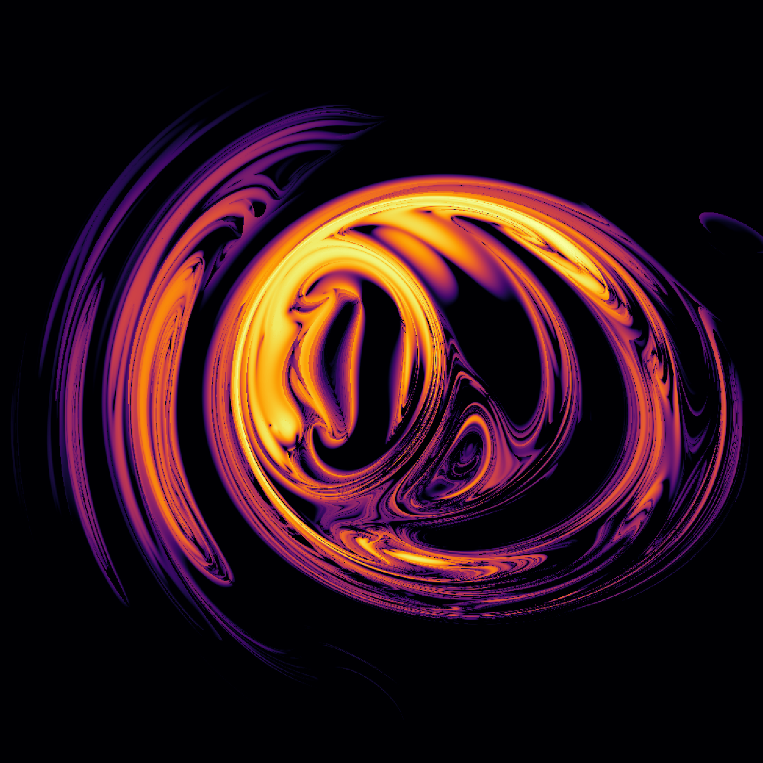
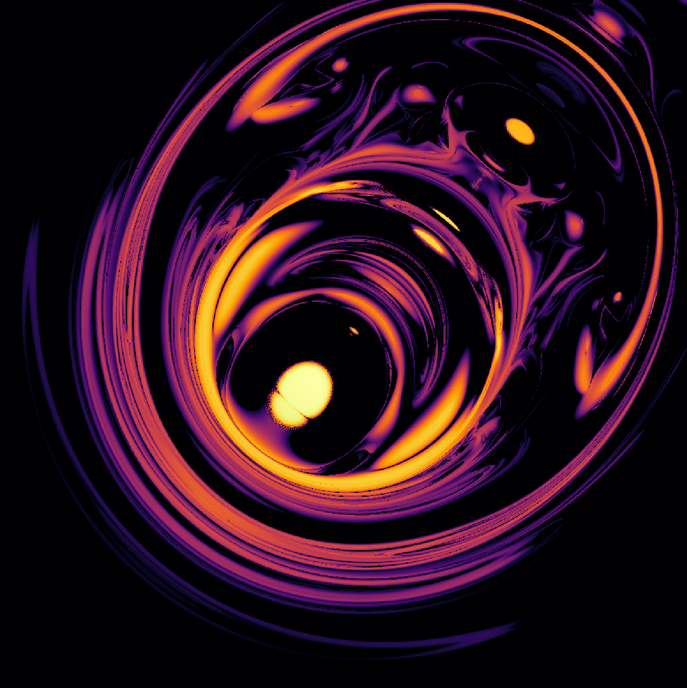
where lighter values indicate earlier divergence. The folded and stretched topology here is known as Smale’s horseshoe, also known as the baker’s dough topology. This map results when a section of space is repeatedly stretched and folded in upon itself, mirroring the process of dough kneading during the bread preparation process. As time goes by, more and more ‘folds’ are apparent, for example as $t_i = 0 \to t_i = 100,000$ we have

If we observe this same plane but starting the planet 1’s z-value at 10.9 and moving to 11.15, we have

It is worth considering what these maps tells us. In a certain region of 2-dimensional space, a planet’s starting point may be shifted only slightly to result in a large difference in the earliest time of divergence. This is equivalent to saying that a planet’s starting point, within a certain region of space, may yield an unpredicable (if it is a point of fast divergence) or relatively predictable (if divergence is slower) trajectory, but even knowing which one of these two possibilities will occur is extremely difficult.

Moreover, knowing which starting points diverge for one set of planets does not allow us to understand which starting points diverge for slightly different planetary masses. If we change the mass of planet 1 from 30 to 5.9 (kg) linearly we have

and changing the force of gravity from $g = 0 \to g = 30.7\; m/s^2$ we have

This topology is not special to points on the $x, y$ plane: on the $y, z$ plane (holding $x=-10$) with $z$ on the vertical axis and $y$ on the horizontal such that the bottom left is $(y, z) = (-20, -20)$ and the top right is $(y, z) = (20, 20)$ after $50,000$ time steps,

Notice something interesting in the $y, z$ divergence pattern that does not exist in the $x, y$ map: a line of mirror symmetry, running from bottom left to top right with a slope of just more than 1. Why does this symmetry exist, and why does it not exist for the $x, y$ map? Most importantly, why are both maps of divergence filled with such intricate detail?

We can address the first question as follows: something must exist in the initial positions of the second and third planets such that symmetry results for the $y, z$ plane but not $z, y$ plane. Thinking about this question in general terms, what would cause our first planet to behave identically with regards to divergence rate at two different locations in space? A readily available answer is that two starting points that result in identical (up to a translation or mirror symmetry) trajectories in space should experience the same divergence rate. After all, if the trajectories are indistinguishable then it would be very strange if one were to diverge faster than the other.

Now consider the placement of planets 2 and 3 in three-dimensional space. Which points on the $y, z$ plane are of equal distance to planets 2 and 3? The answer is the points that are equidistant from any certain point on the line connecting planets 2 and 3, projected onto the $y, z$ plane. Each pair of points in the $y, z$ plane that are equidistant from any point on this line will thus have identical trajectories, and should therefore have equal divergence which follows from our earlier argument.

Is this the case? Recalling that the initial points for planet 2 and planet 3 are

\[(p2_x, p2_y, p2_z) = (0, 0, 0) \\ (p3_x, p3_y, p3_z) = (10, 10, 12)\]

the line connecting these points projected onto the $y, z$ plane has the equation $z=(12/10)y$. Plotting this line together with the map formed by observing divergence in the $y, z$ plane for $x=-10$, we see that indeed this is our line of mirror symmetry:

Why does our $x, y$ plane not exhibit such symmetry? After all, projecting the line connecting p2 and p3 onto the $x, y$ plane we have $y=x$ so why is there no line of symmetry about the diagonal? This is because the initial velocites for both p1 as well as p3 contain non-zero components of $x$. Now imagine any two initial points that are equidistant from a point on the line $y-x$. Are the trajectories of these two points still identical given that they have different identical but non-zero starting velocities in the $x, y$ plane? They are, because for one point of the pair the initial velocity vector will cause the approach to the line of symmetry to come sooner, whereas for the other point it will be longer or may not occur at all.

To begin to answer the second question of why such detailed shapes form when we plot divergence time, one can ask the following: which initial points of the $y, z$ plane land close to the line of symmetry as the planets move over time? Because the trajectory of all three bodies are completely determined by their initial positions (and velocities), for any initial value of $y_0, z_0$ that approaches the line of symmetry such that $(12/10)y_i - z_i < \delta$ then the initial value’s mirror point $y’_0, z’_0$ also approaches the line, as the trajectories and distances to that line are identical for these initial points.

Thus although could very well pick any other region to investigate the question of which initial points (for p1) end up there at any time, the region of initial mirror symmetry has one important simplifying aspect: the resulting map will stay symmetric about the initial line of symmetry, making it easier to see where the points are located.

The code to plot this is as follows:

def plot_projection(self, divergence_array, i):
	...
	divergence_array[(self.p1[1] * 12 - self.p1[2] * 10 < 1).numpy() & (self.p1[1] * 12 - self.p1[2] * 10 > -1).numpy()] = i
	plt.imshow(divergence_array, cmap='inferno', extent=[-20, 20, -20, 20])
	plt.axis('on')
	plt.xlabel('y axis', fontsize=7)
	plt.ylabel('z axis', fontsize=7)
	plt.savefig('Threebody_divergence{0:04d}.png'.format(i//100), bbox_inches='tight', dpi=420)
	plt.close()

such that each initial point in the $y, z$ plane that is close to (specifically within 2 units using the Manhattan distance metric) of the line $z=(12/10)y$ appear as white spots. At $t=50,000$, the map is as follows

Now we can attempt to understand how the divergence map attains the horseshoe topology by observing the points that are mapped to our line of symmetry over time, as the horseshoe map itself forms over time. The points which map to the line $z=(12/10)y$ exist on a relatively stable manifold. Why is the line of symmetry relatively stable?

We can see that indeed the initial points which map to the line of symmetry also tend to be stable by simply observing that in our figure, the white points mostly occupy the dark regions in the divergence map. But why is this the case? All points starting exactly on the line of symmetry (meaning that p1 starts on any point where $10z = 12y$) will remain on this line because in that case all three planets exist in a plane, and with no initial velocity in the $y, z$ plane they will stay in that plane and thus are accurately modeled in two dimensions. This means that their trajectories will be periodic (see the next section for more details) and therefore divergence will not occur, making these starting points stable.

What about the case for trajectories of p1 that reach the line of symmetry after some time, why do they tend to be more stable? We now have a far more difficult question to address, but for an investigation into one- and two-dimensional analogues of that question this page.

Observing as $t_i=0 \to t_i=87,800$ we have:

Notice how these points on a stable manifold continually intersect, or more accurately meet and become repelled by unstable regions such that they elongate and gradually form a web-like mesh. This dynamic structure was termed a ‘homoclinic tangle’ by Poincaré, and was later shown by Smale to imply and be implied by the horseshoe map.

To see what happens when we observe a different region, here is the map of which initial points are located near the line $z=(12/10)y + 3$ at any given time from $t_i=0 \to t_i=150,000$

So in one sense, the regions of quickly- and slowly-diverging points are arranged in such a complicated and detailed fashion because they result from the continual mixing of stable (slowly diverging) and unstable (quickly diverging) regions of space.

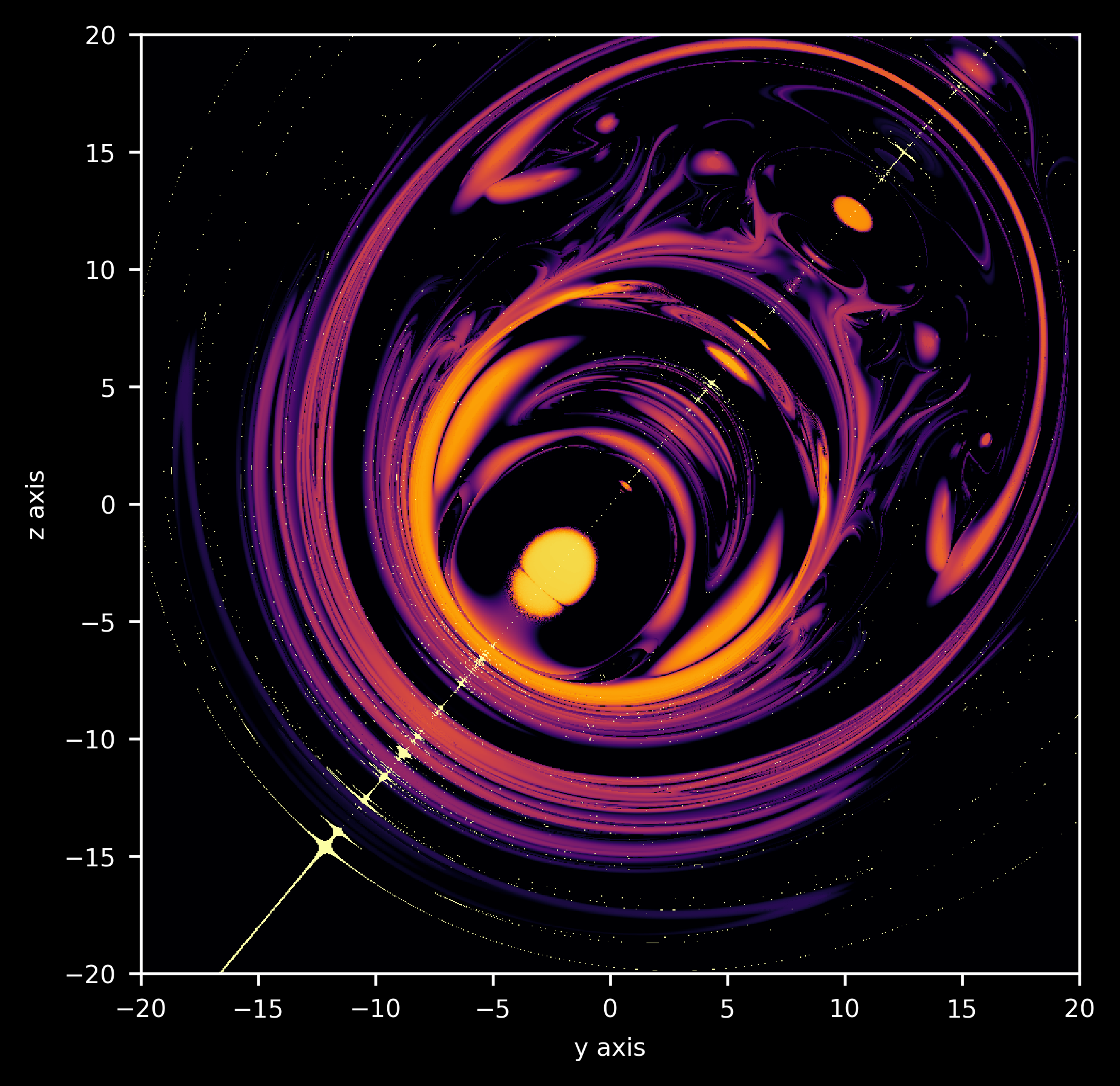
We can also ask which points in the $y, z$ plane end up in an arbitrary region, and not limit ourselves to lines near our line of symmetry. Observing which points map to the interior of a circle of radius $5$ centered on the point $y, z = 20, 10$ we have

This clearly shows us how for the three body system, space is stretched and folded. Stretched here is where approximate circles are flatten out and elongated, and folded is where new regions mapped to our circle seem to appear out of nothing.

Is there a specific region in which initial positions that have diverged are more likely to be found compared to positions of planet 1 that have not diverged? One guess is that trajectories in which planets that are ‘ejected’, ie sent far away from each other, are those for which the divergence is more likely to occur. We can plot the initial points where planet 1 is at least 150 units from the origin in white as follows:

Which suggests that some but not all ejected trajectories are also diverged, and on the other hand some non-diverged trajectories are also those that experience ejection.

Two body versus three body problems

How does this help us understand the difference between the two body and three body problems? Let’s examine the two body problem as a restricted case of the three body problem: the same differential equations used above can be used to describe the two body problem simply by setting on the of masses to 0. Lets remove the first object’s mass, and also change the second object’s initial velocity for a trajectory that is easier to see.

# masses of planets
m_1 = 0
m_2 = 20
m_3 = 30

...

# p2_start = x_2, y_2, z_2
p2_start = np.array([0, 0, 0])
v2_start = np.array([-3, 0, 0])

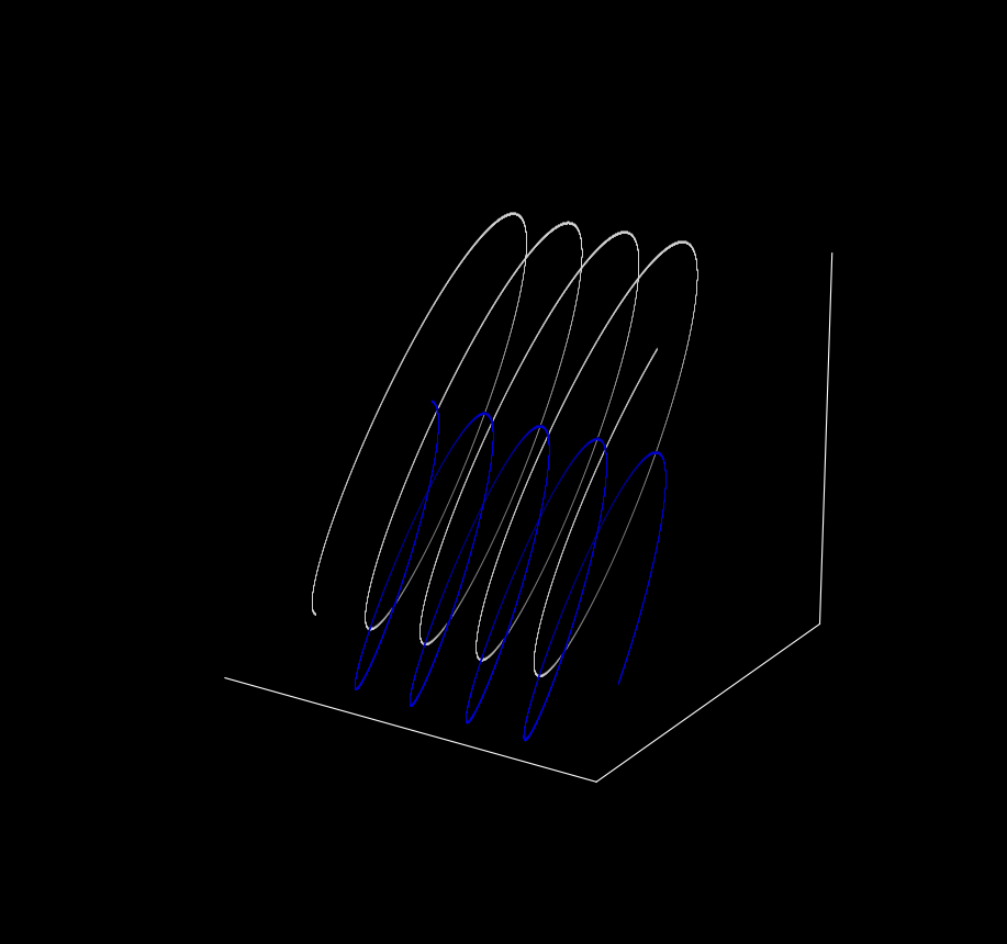
Plotting the trajectories of p2 and p3,

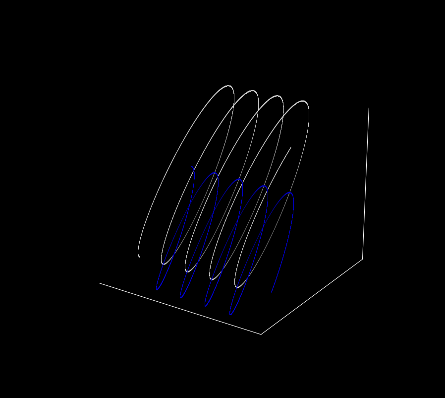
This plot looks much more regular! As we will later see, these trajectories form periodic orbits that, like other two body trajectories, lie along a plane. We can do some fancy rotation in three dimensional space by changing using a second loop after our array-filling loop to show this.

...

for t in range(360):
	fig = plt.figure(figsize=(10, 10))
	ax = fig.gca(projection='3d')
	plt.gca().patch.set_facecolor('black')
	
	plt.plot([i[0] for i in p2], [j[1] for j in p2], [k[2] for k in p2] , '^', color='white', lw = 0.05, markersize = 0.01, alpha=0.5)
	plt.plot([i[0] for i in p3], [j[1] for j in p3], [k[2] for k in p3] , '^', color='blue', lw = 0.05, markersize = 0.01, alpha=0.5)

	plt.axis('on')
	# optional: use if reference axes skeleton is desired,
	# ie plt.axis is set to 'on'
	ax.set_xticks([]), ax.set_yticks([]), ax.set_zticks([])

	# make panes have the same color as the background
	ax.w_xaxis.set_pane_color((0.0, 0.0, 0.0, 1.0))
	ax.w_yaxis.set_pane_color((0.0, 0.0, 0.0, 1.0))
	ax.w_zaxis.set_pane_color((0.0, 0.0, 0.0, 1.0))
	
	ax.view_init(elev = 20, azim = t)
	plt.savefig('{}'.format(t), dpi=300, bbox_inches='tight')
	plt.close()
	

An aside: aren’t trajectory crossings impossible for ordinary differential equations? For the case of a single object moving in space, this is correct, because any trajectory crossing would imply that some point heads toward two different points next, an impossibility for any function. But as we have two objects, each with velocity as well as position vectors, crossings can occur if the other object is in a different place than before. On the other hand, it would be impossible for the two planets to occupy the same position they held previously, with the same velocity vectors, without re-visiting future points.

Now let’s see what happens when we shift the starting value of one of the points by the same amount as before ($z_3 = 12 \to z_3 = 12.000001$).

The trajectories looks the same! When both original and shifted trajectories of the $p_2$ are plotted, it is clear to see that there is no separation ($z_3 = 12$ in white and $z_3 = 12.000001$ in blue)

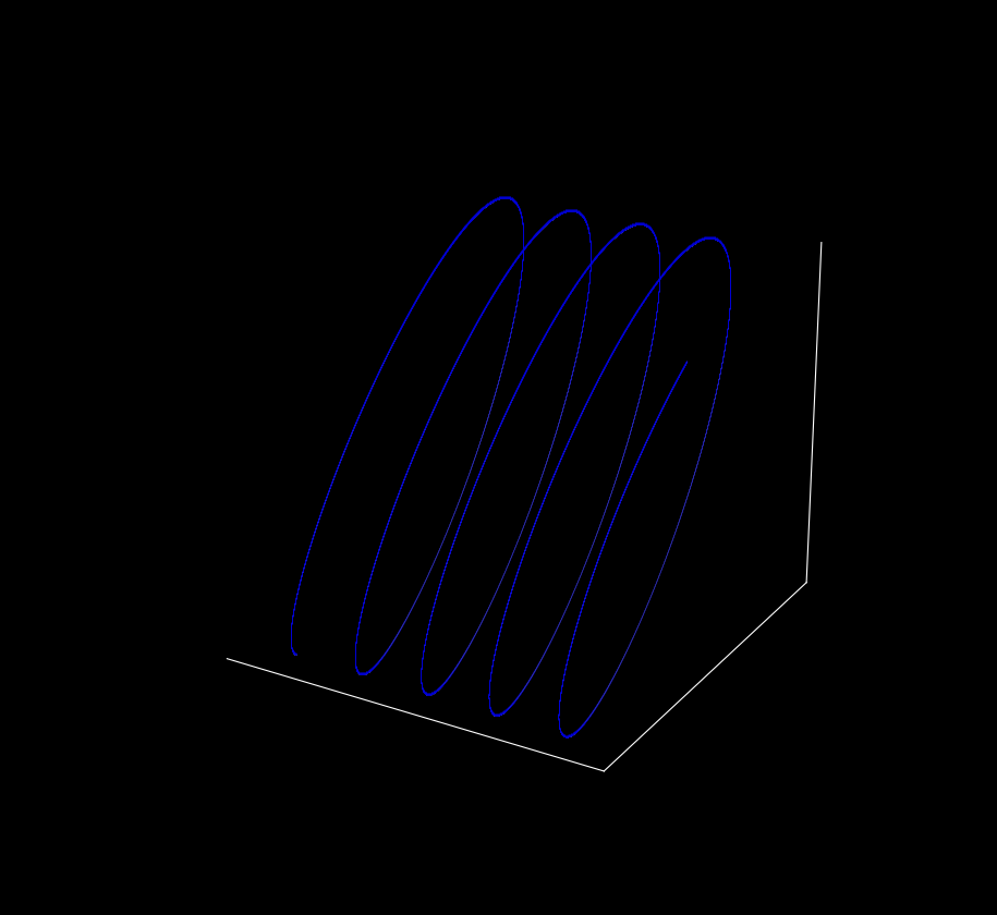
This means that this trajectory of a two body problem is not sensitive to initial conditions: it is not chaotic. Is this always the case regardless of the initial positions and velocities? Indeed it is, as by the Poincaré-Bendixson theorem all continuous trajectories in two dimensions are periodic. As was later shown by Lorenz and others, periodicity implies insensitivity to initial values and thus no two-dimensional continuous map can be chaotic.

Thus it turns out that periodicity (and asensitivity to initial values) is the rule for all two body problems: all are periodic or quasi-periodic, meaning that future trajectories are identical to past trajectories. This means that we can remove (all but a negligable amount) of the time variable when we integrate these differential equations.

On the other hand, most (all but a miniscule number of) three body trajectories are aperiodic. And this in turn means that their future trajectories are never exactly like previous ones such that we cannot remove time from the differential equations. This makes them unsolvable, with respect to a solution that does not consist of adding up time steps from start to finish.

The three body problem is general

One can hope that the three (or more) body problem is restricted to celestial mechanics, and that it does not find its way into other fields of study. Great effort has been expended to learn about the orbitals an electron will make around the nucleus of a proton, so hopefully this knowledge is transferrable to an atom with more than one proton. Unfortunately it does not: any three-dimensional system with three or more objects that operates according to nonlinear forces (gravity, electromagnetism etc.) reaches the same difficulties outlined above for planets.

This was appreciated by Feynman, who states in his lectures (2-9):

“[Classical mechanics] is deterministic. Suppose, however, that we have a finite accuracy and do not know exactly where just one atom is, say to one part in a billion. Then as it goes along it hits another atom…if we start with only a tiny error it rapidly magnifies to a very great uncertainty…. Speaking more precisely, given an arbitrary accuracy, no matter how precise, one can find a time long enough that we cannot make predictions valid for that long a time”

The idea that error magnifies over time is only true of nonlinear systems, and in particular aperiodic nonlinear systems. On this page, we have seen that in a nonlinear system of two planets, error does not magnify whereas it does for the cases observed with three planets. Therefore measurement error does not necessarily become magnified, but only for aperiodic dynamical systems. This was the salient recognition of Lorenz, who found that aperiodicity and sensitivity to initial conditions (which is equivalent to magnification of error) implied one another.

Does it matter that we cannot solve the three body problem, given that we can just simulate the problem on a computer?

When one hears about solutions to the three body problem, they are either restricted to a (miniscule) subset of initial conditions or else are references to the process of numerical integration by a computer. The latter idea gives rise to the sometimes-held opinion that the three body problem is in fact solveable now that high speed computers are present, because one can simply use extremely precise numeric methods to provide a solution.

To gain an appreciation for why computers cannot solve our problem, let’s first pretend that perfect observations were able to be made. Would we then be able to use a program to calculate the future trajectory of a planetary system exactly? We have seen that we cannot when small imperfections exist in observation, but what about if these imperfections do not exist? Even then we cannot, because it appears that Newton’s gravitational constant, like practically all other constants, is an irrational number. This means that even a perfect measurement of G would not help because it would take infinite time to enter into a computer exactly.

That said, computational methods are very good for determining short-term trajectories. Furthermore, when certain bodies are much larger in mass than others (as is the case in the solar system where the sun is much more massive than all the planets combined), the ability to determine trajectories is substantially enhanced. But like any aperiodic equations system, the ability to determine trajectories for all time is not possible.