Entropy Estimation Models

This page is best viewed with FireFox, as most other popular browsers (Chrome, Safari etc.) will not render the MathJAX correctly.

Introduction

In work detailed in a blog post and paper, a major finding was that one can modify a new causal language model architecture termed the ‘masked mixer’ (which is essentially a transformer with self-attention replaced by masked 1D convolutions) to effectively autoencode inputs with high compression, that is, one can train small models in reasonable time to be able to regenerate (with some error) a sequence of 512 or more tokens using the embedding of only one token with excellent generalization properties. It was found that using masked mixers for encoder and decoder allows for far greater input autoencoding accuracy than a transformer encoder/decoder pair for a given model size ad compute budget during training, leading to the ability to compress inputs using new and potentially more efficient methods than what has been possible using the transformer.

It may be wondered why text compression ability is important: even if large language models achieve 2x or 4x the compression of commonly used algorithms like gzip, they are thousands of times more computationally expensive to actually run and thus not preferred today (although this may change in the future). The answer is that effective compression from many to one token allows one to design architectures that have interesting properties such as extended context windows or meta-context guidance, which we will investigate under the broad name of ‘memory’.

We will first tweak the autoencoder mixer architecture to try to obtain optimal text compression in fixed compute budgets before using this information to attempt to test whether one can obtain better text compression ratios than the current best methods (which are large causal language modeling transformers). We will conclude by examining the suitability of autoencoding embeddings for extending generative language model context with sub-quadratic complexity using encoder embeddings.

Transformer-based autoencoders train and scale poorly

In previous work evidence was presented for the idea that masked mixers were far better autoencoders than transformers, with the primary large-scale data evidence being the following: if one trains a $d_m=1024$ masked mixer autoencoder with $n_l=8$ layers in the encoder and decoder, one reaches a far lower CEL than the compute- and memory- transformer model with $d_m=512$ (transformers contain far more activations per $d_m$ due to their $K, Q, V$ projections). One may object that this could be mostly due to differences in the amount of information available in a 512-dimensional vector compared to a 1024-dimensional vector, although that was not found to be the case on the much smaller TinyStories dataset where equivalent-dimensional transformers far underperformed their masked mixer counterparts despite requiring around double the compute and device memory.

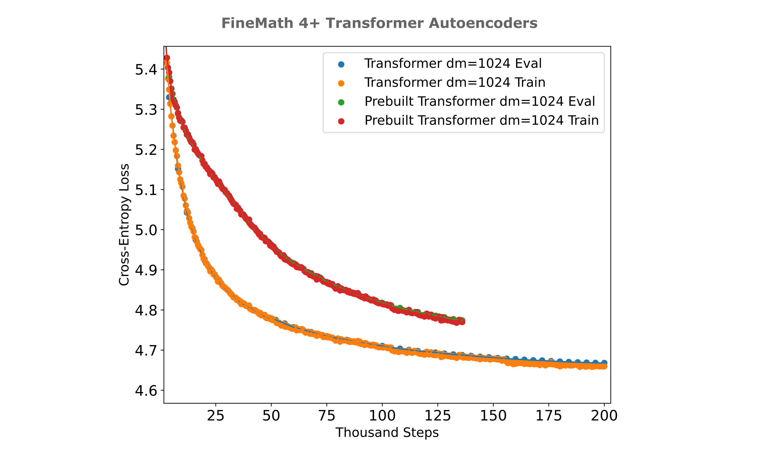
We are in a position to now further explore the training efficiencies for transformer-based versus mixer-based autoencoders. Perhaps the first question one might have when observing the very large performance gap between transformer and mixer is if there is some implementation error in the transformer architecture. The original implementation used pre-built Llama model blocks from the Huggingface transformers library, and implemented loops through these blocks for encoder and decoder while using the same vector broadcasting and tensor rearrangements, word-token embedding, and language modeling heads transformations as the masked mixer counterpart, feeding the positional information to each layer. It may be wondered if a much simpler implementation would perform better, where the encoder and decoder are each LlamaModel transformer implementations, and we also include an attention mask on the decoder. From the figure below, we can see that the transformer autoencoder with pre-built encoder and decoder is actually somewhat worse than the original modular architecture when trained on the FineMath 4+ dataset.

The other main oustanding question is whether the increased masked mixer autoencoder training efficiency might be due to the larger embedding dimension in that model versus the transformer, at least for larger and more diverse datasets like finemath 4+ or fineweb-edu. This is primarily a scaling question with respect to increases in the model $d_m$ (and thus the embedding dimension in this case), so one can obtain a more general idea of the differences in masked mixer versus transformers for autoencoder training efficiency by comparing the losses achieved as one scales the model $d_m$ for a given training dataset.

From the following figure, it can be appreciated that indeed transformers are far less efficient to train as autoencoders than masked mixers for multiple $d_m$ values, providing evidence for the idea that differences in autoencoding abilities between these models are not due to those differences but are instead model intrinsic (specifically attention-intrinsic). For context, we have a total of $n = 200,000 * 128 * 512 \approx 13.1 * 10^9$ tokens trained at 200k steps for each model in the following figure.

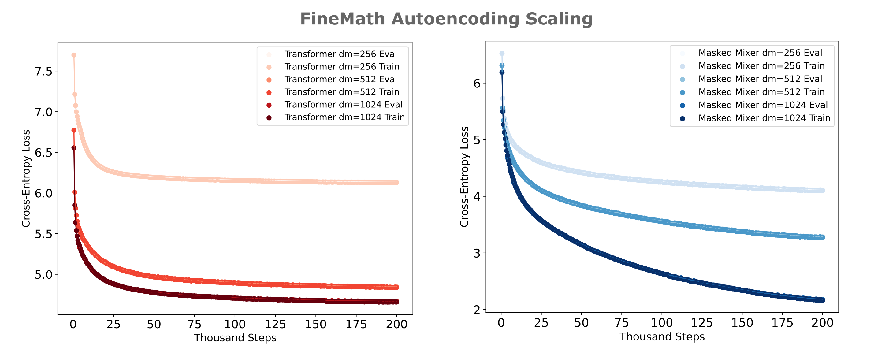
It is apparent that transformers scale badly in terms of samples per model, as apparent by the negative asymptotic slope of the transformer training curves being far smaller than that of the masked mixer. Transformers-based autoencoders also scale poorly in terms of scaling the embedding size or equivalently the model width, which is apparent as doubling the $d_m$ of a transformer autoencoder twice gives decreasing loss achieved with each doubling, whereas the opposite is true for masked mixer autoencoders.

None of this is particularly surprising given the results and theory outlined in the masked mixer introductory paper. One major finding there is that transformers are relatively inefficient to train for tasks requiring retention of information present in the input, either in a single or multiple output embeddings.

Why transformers struggle with repeated embeddings

From the last section we observed that transformers make far worse autoencoders (with the architecture presented at least) than masked mixers. The next question to ask is why this is: why would transformers be so much worse than masked mixers, given that in previous work has shown more modest differences in information retention between transformers and masked mixers? More specifically, why would attention lead to poor autoencoding in this architecture?

Some reflection will provide a reasonable hypothesis: recall that attention may be expressed as follows:

\[A(Q, K, V) = \mathrm{softmax} \left( \frac{QK^T}{\sqrt(d_k)} \right)V\]

where the $Q, K, V$ are matrices of packed vectors projected from each token embedding. To make these operations clearer from the perspective of token indices, we can ignore the $d_k$ scaling factor and express this equation as follows: the attention between the query projection for token $i$ and key and value projections at index $j$, for ${i, j \in n}$ is

\[A(q_i, k_j, v_j) = \frac{\exp \left( (q_i \cdot k_j) v_j \right)}{ \sum_n \exp \left( (q_i \cdot k_n) v_n \right)}\]

Now consider what we have done by repeating the input embedding for all tokens in the decoder: as the projection weight matrices $W_k, W_q, W_v$ are identical for all tokens, the necessarily we have the following:

\[k_i = k_j \\ q_i = q_j \\ v_i = v_j \forall i, j\]

and thus $q_i \cdot k_j = q_i \cdot k_l \; \; \forall i, j, l$. Therefore we have $A(q_i, k_j, v_j) = A(q_i, k_l, v_l) \; \forall i, j, l$ such that output activations from the attention layer are identical across all token embeddings.

Given this observation, it is not hard to see that this identicality will persist for more than one layer as each feedforward module following attention is identical. But this is not the whole picture: as implemented, Llama-style transformers apply positional encoding (RoPE in this case) before self-attention such that the embeddings at each position are actually unique, assuming that the positional encoding is itself unique for the token indices we are training on (on this page it always will be). Thus is is not strictly correct to point to identical activations due to self-attention as being the cause of the poor transformer training for repeat-embedding autoencoders, but one might wonder whether perhaps transformers are less well-suited to autoencoding with repeated embeddings relative to masked mixers.

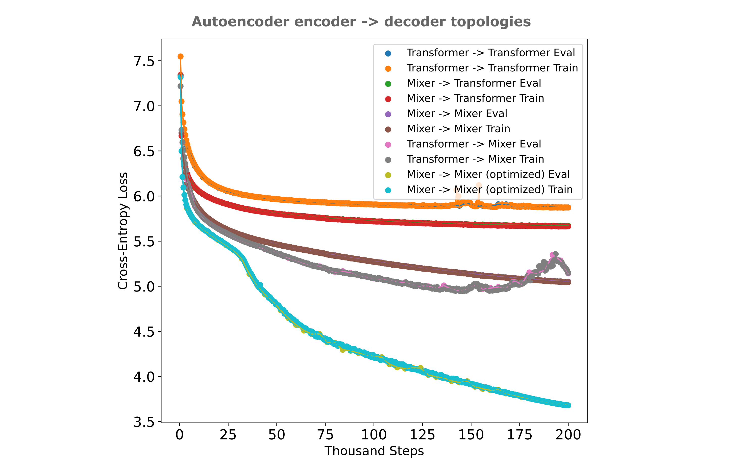
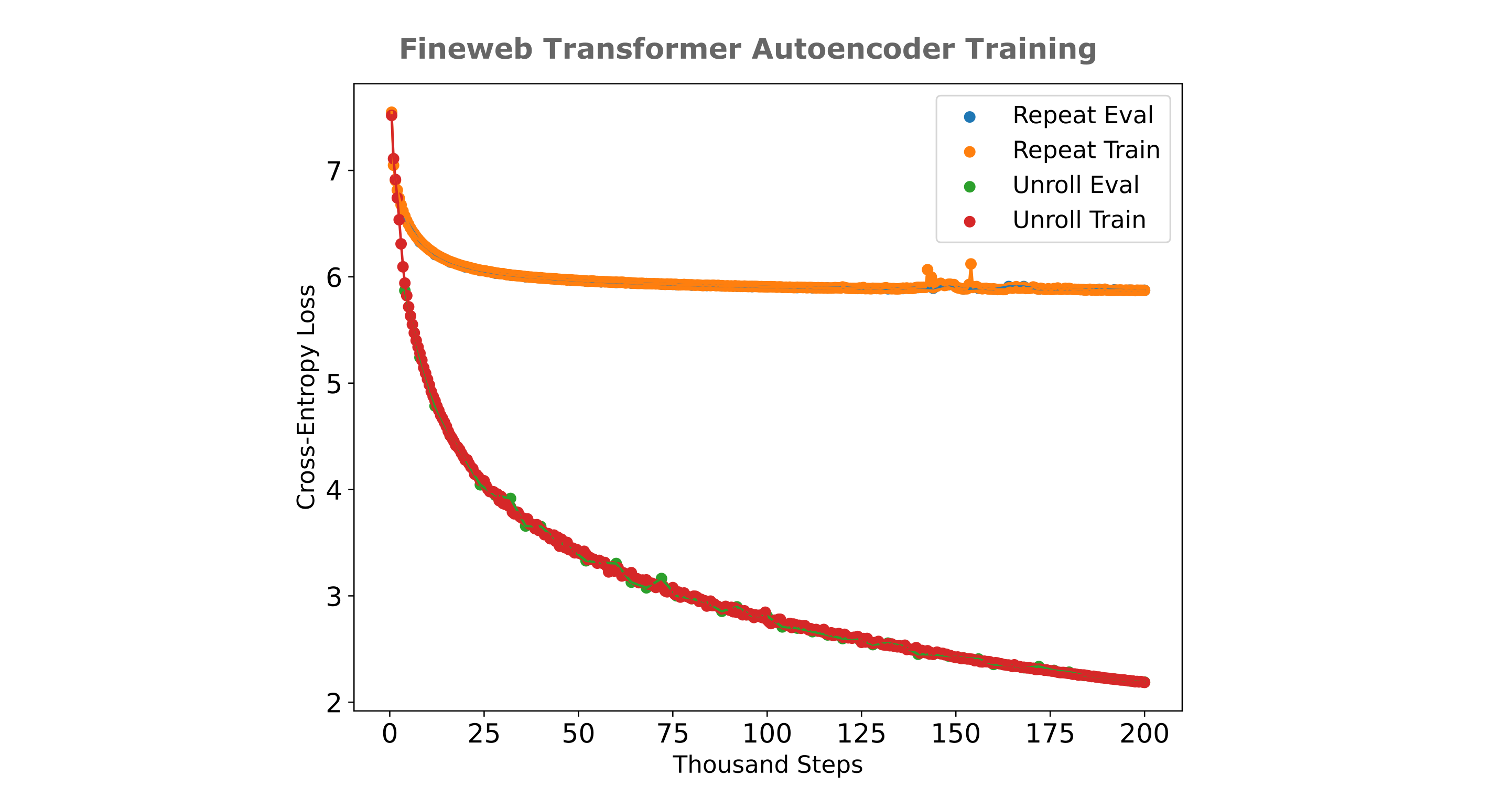
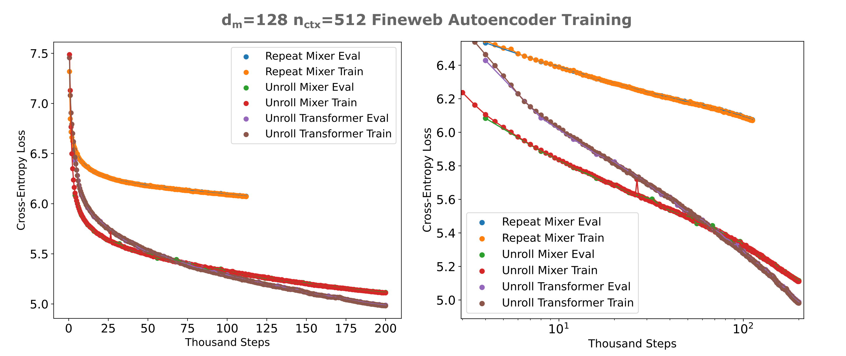
One indirect way we can test this is as follows: if a transformer were significantly worse for decoding repeated embeddings than a masked mixer, we would expect for an autoencoder with a mixer encoder and transformer decoder to perform worse than an autoencoder with a mixer encoder and decoder, or an autoencoder with a transformer encoder and mixer decoder. As shown in the following figure, this is indeed what is found (although an optimized masked mixer autoencoder is more efficient than either compound architecture).

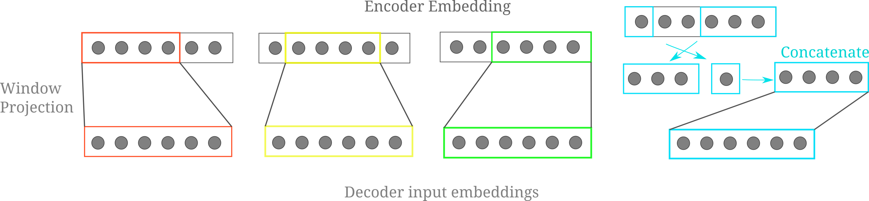
Given some evidence for our idea, how would one go about injecting an encoder’s embedding to a transformer decoder while avoiding the identical attention problem? One simple but effective way to do this is to ‘unroll’ the embedding by projecting unique subsets of the encoder’s embedding into each of the decoder’s input positions. A relatively simple but flexible method to get unique subsets of a vector is to use a sliding window, where we project from a certain number of contiguous elements of a vector in our ‘window’ and shift the elements projected from at each of the decoder’s indices, keeping the projection weights identical across all input windows. This requires an embedding vector satisfying $d_m \geq n_{ctx}$ for every decoder index vector to be unique, but we can simply add a projection to enlarge the $d_m$ of the embedding as required if necessary.

For cases where we want to project from $n_d$ elements and $d_m < n_d + n_{ctx} - 1$, or in other words where our window slides off our embedding vector to make all decoder inputs, we can simply wrap our window around to the first index of the embedding, concatenate, and project accordingly. For the case where $n_{ctx}=4, d_m=6, n_d = 4$, the following diagram illustrates the projection and wrapping process:

This approach can be generalized to inputs of arbitrary token length by re-assigning the slice indices to be the modulo division remainder of the index and the embedding dimension. We implement as follows: given a linear projection layer that assumes the input is half the size of the ouput, self.projection = nn.Linear(dim//2, dim), we can replace the embedding repeat with our unrolled projections

encoder_embedding = x[:, -1, :].unsqueeze(1) # dim=[batch, token, hidden]
embedding_stack = []
# sliding window unroll over hidden dim
for i in range(self.tokenized_length):
    index = i % dim
    sliding_window = encoder_embedding[..., index:index+dim//2]
    if index+dim//2 > dim:
        residual = index+dim//2 - dim
        # loop around to first index
        sliding_window = torch.cat((sliding_window, encoder_embedding[..., :residual]), dim=2)
    embedding_stack.append(sliding_window)
encoder_embedding = torch.cat(embedding_stack, dim=1)
encoder_embedding = self.projection(encoder_embedding)

Note here that an implementation most faithful to our figure above would be to apply the projection at each index in the for loop before concatenation, but this is much less efficient as applying the projection to the pre-concatenated output allows us to make use of device (GPU) parallelization that is otherwise tricky to add to the loop via Pytorch primitives.

The exact token indices that we use for the wrap are not important: we observe essentially identical results if we use a middle-out approach rather than a wrap-to-front, which can be implemented by residual = index+dim//2 - dim//2.

For a $d_m=512, n_l=8$ (eight layer for encoder, eight for decoder) applied to $n_{ctx}=512$ FineWeb-edu, we have the following:

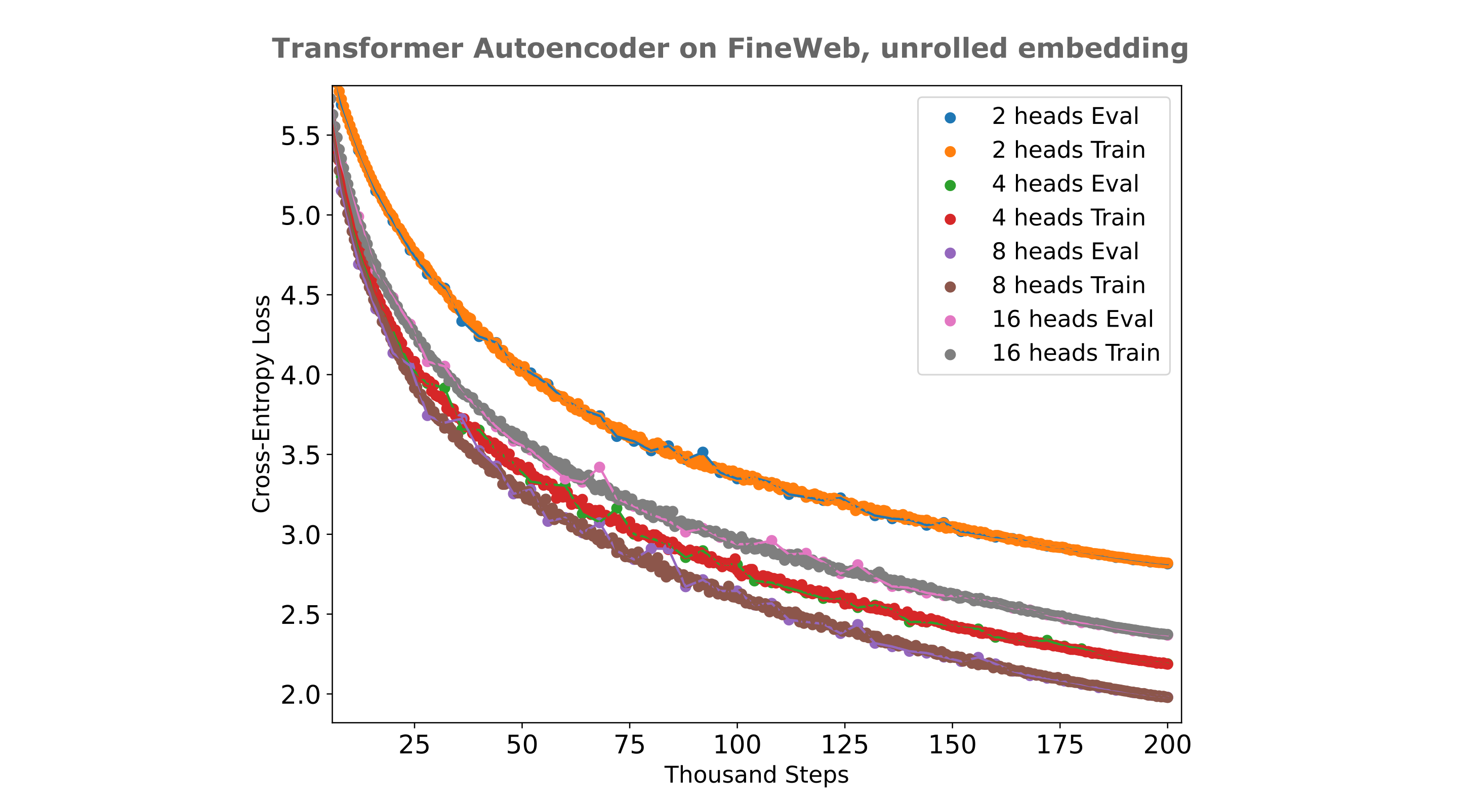
We can also take the effort to find the optimal number of heads for our autoencoder, and the figure below shows the training efficiencies for various head sizes. It can be appreciated that eight heads are optimial or near-optimal for this autoencoder using the unrolled embedding technique.

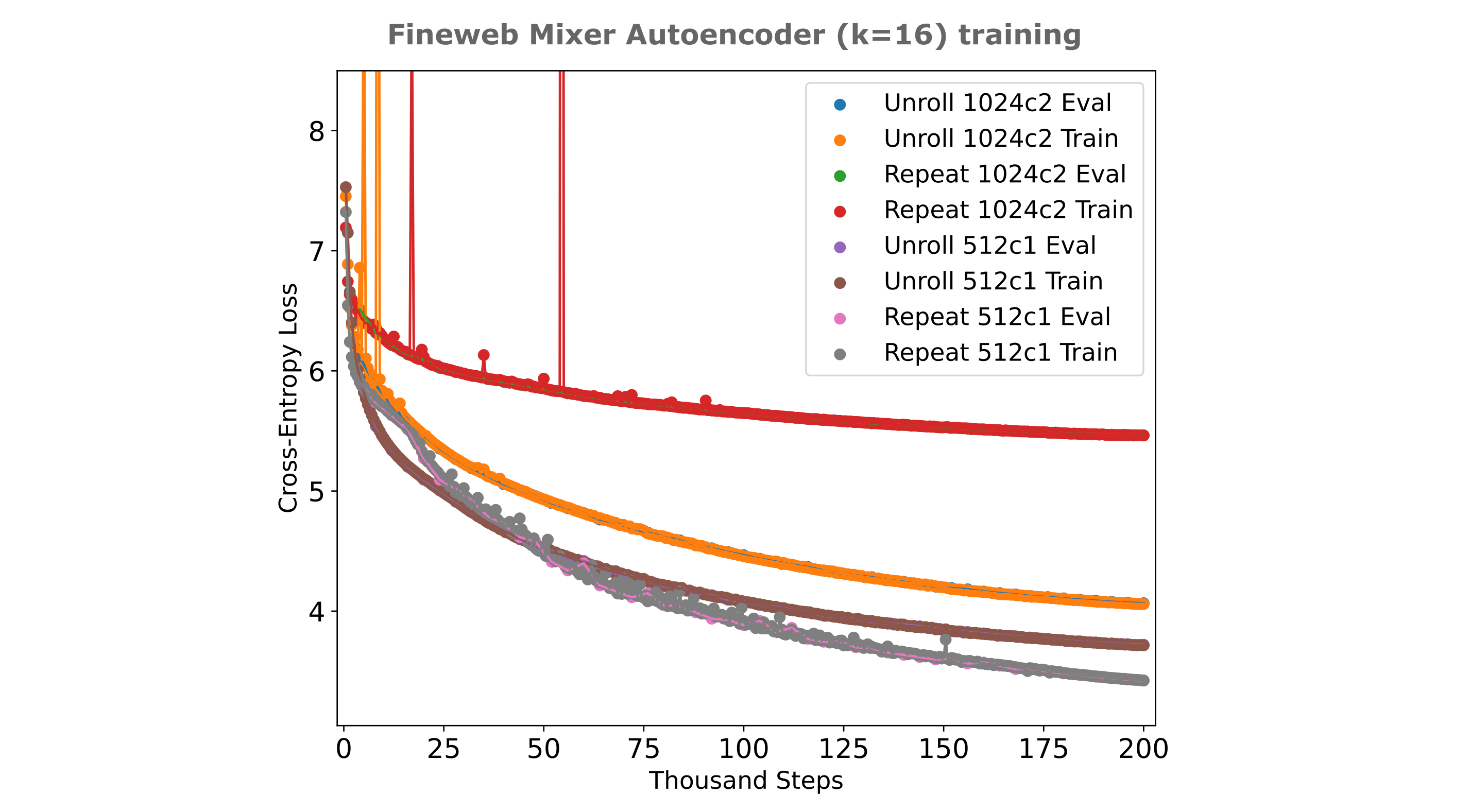
Does the use of unrolled embeddings lead to masked mixer autoencoders training more efficiently? The answer is generally not at one $d_m$: for the most performant convolutional kernel sizes, the use of repeated embeddings leads to more efficient training.

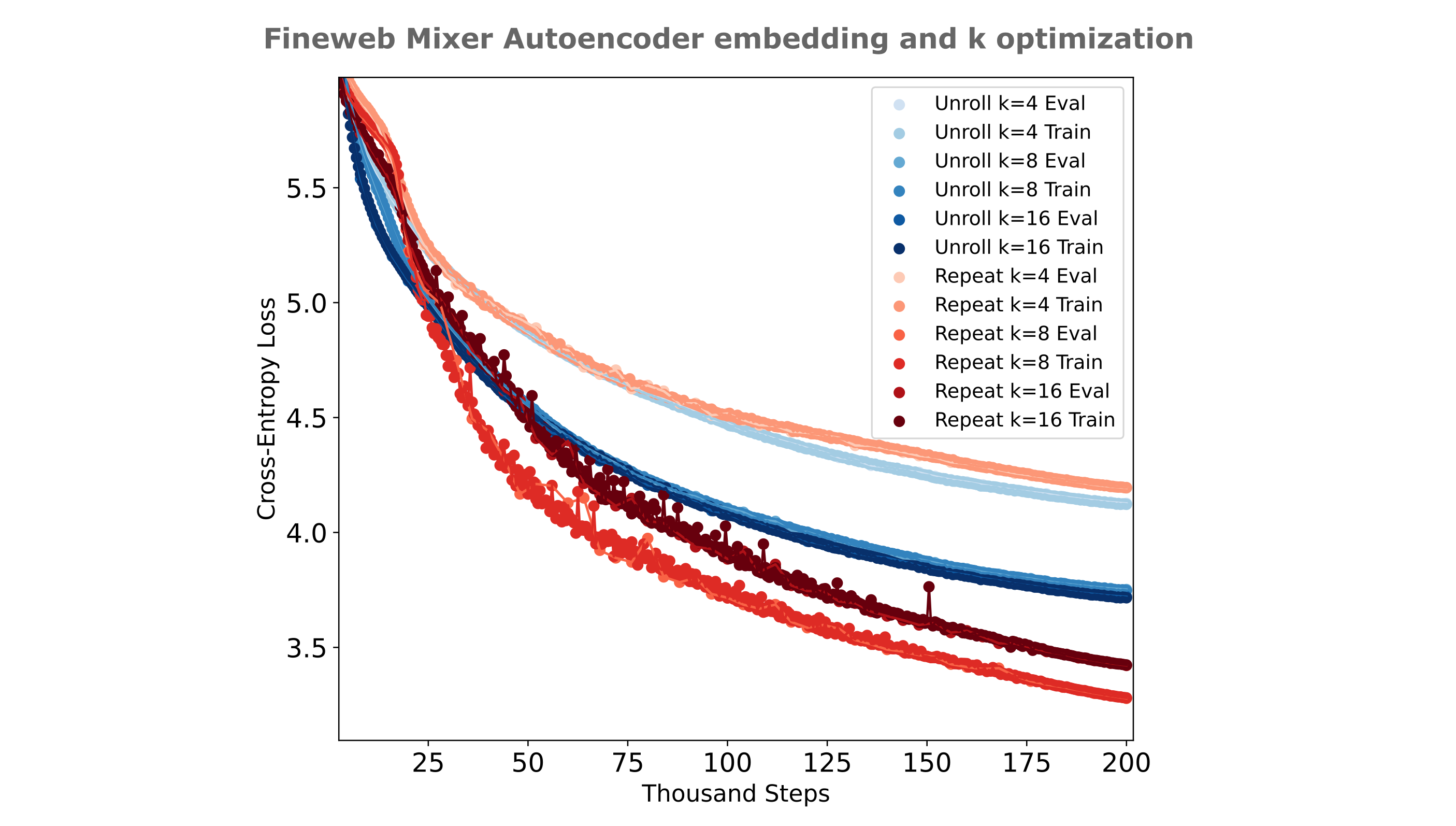
It is interesting, therefore, that for a model with a larger embedding ($d_m=1024$) we find that this is not the case:

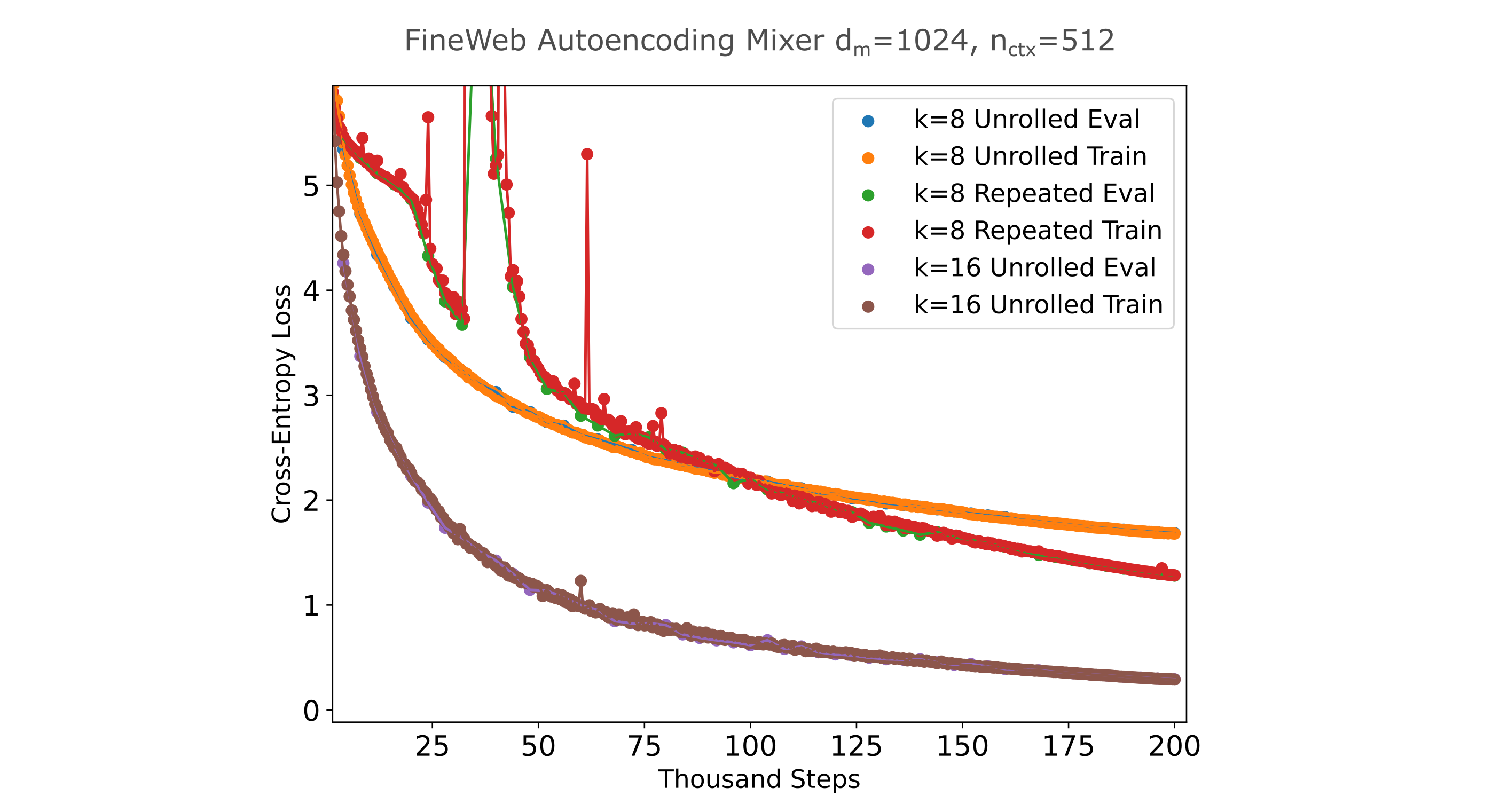
It should be noted that the masked mixers in the above figure use around half the compute and device memory as the transformers in the figure before, and cannot be compared directly for training efficiency purposes. It is interesting to note that expanding the transformer width and using a compression layer (two linear transformations that compress $d_m \to d_m/2 \to d_m$ lead to substantially worse training efficiency than using a smaller $d_m$ with no compression between encoder and decoder, despite the smaller-$d_m$ model requiring half the compute and memory to train.

Causal masking increases autoencoder training efficiency

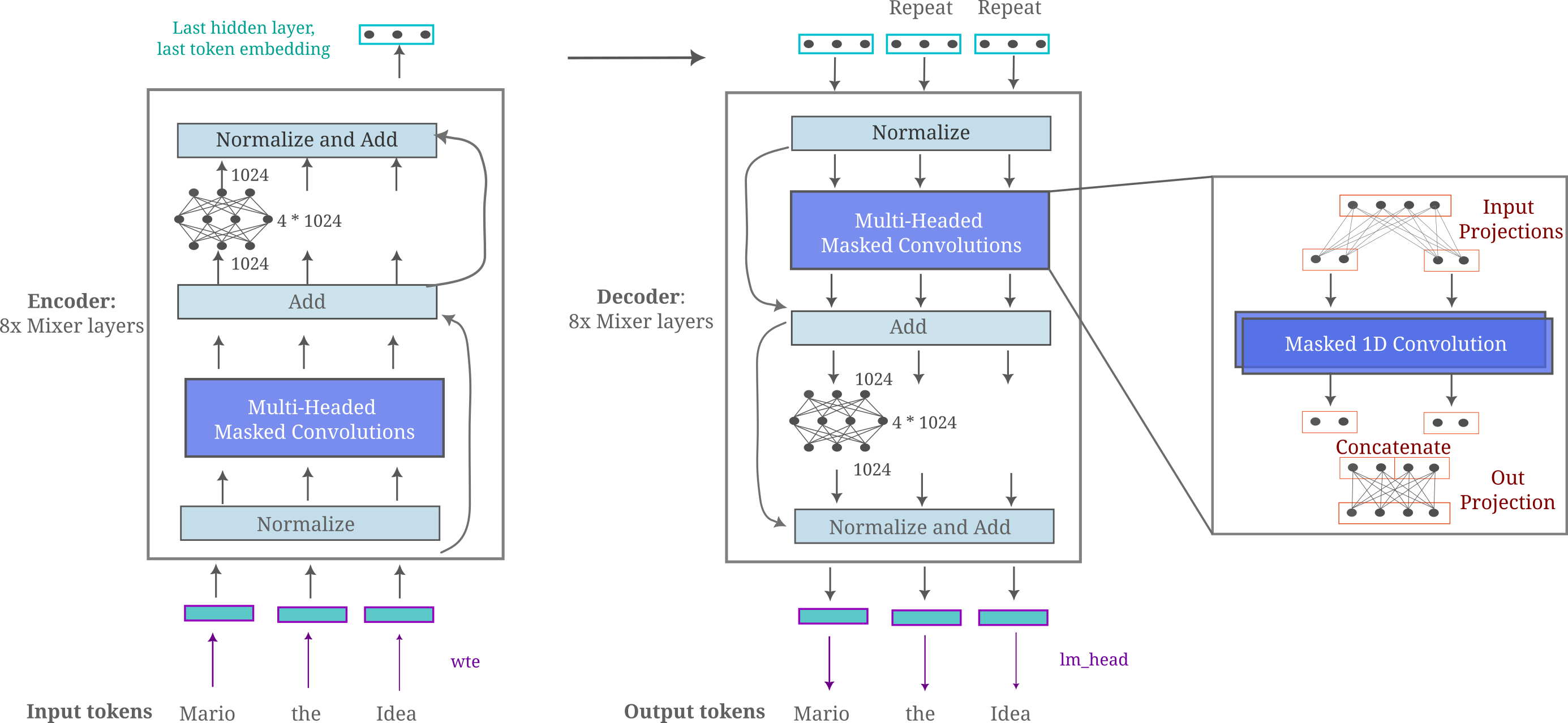
To begin with, it is helpful to recall the architecture of the masked mixer-based autoencoder as presented in the work linked in the last section:

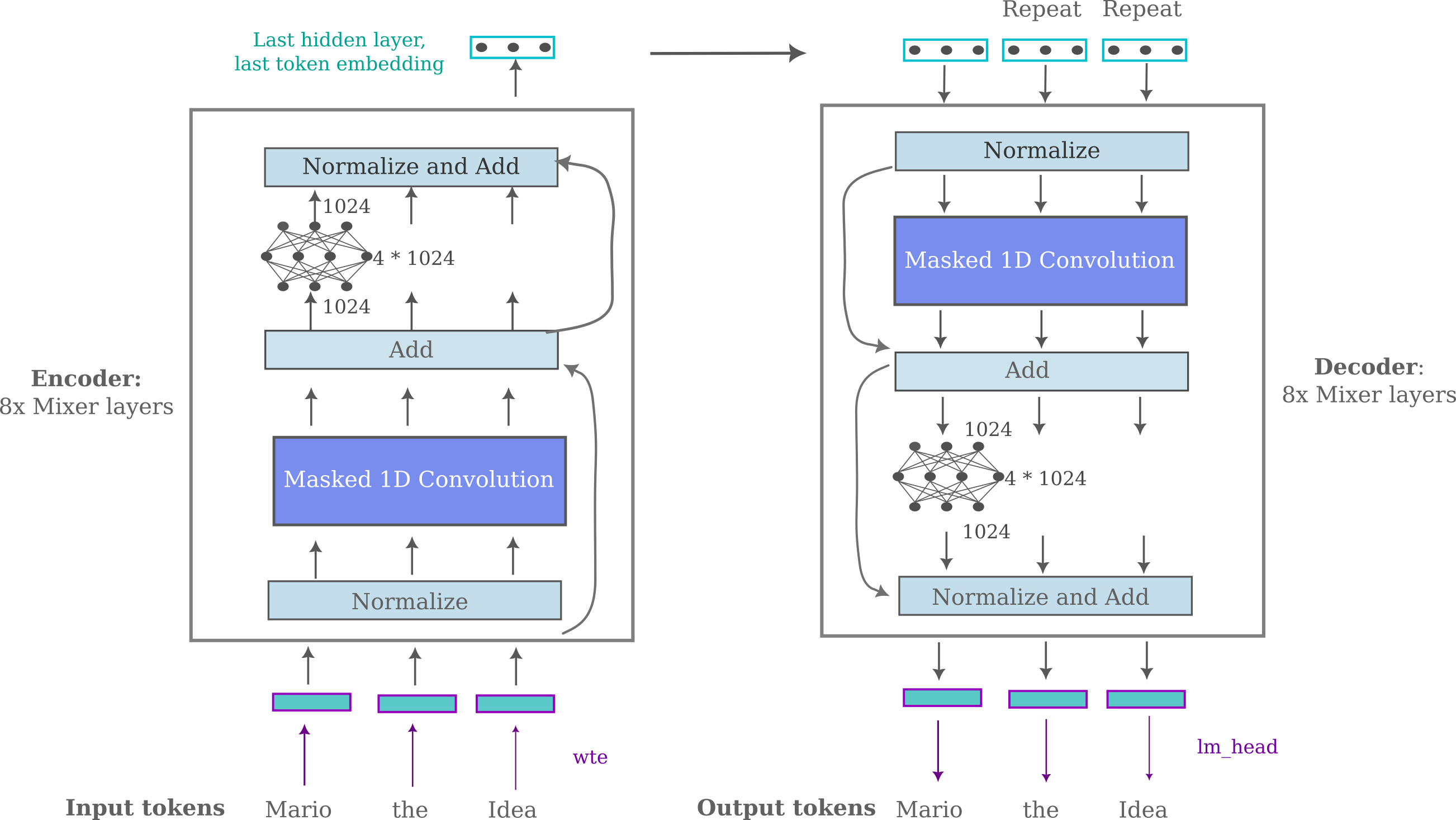
This architecture recieved little to no optimization in that work, as it was mostly presented as evidence for a hypothesis involving bijective functions and autoencoding. But now that we want to improve and elaborate upon this architecture, where would we start?

One obvious question is whether or not the convolutions really need to be masked: after all, we are generating the output in one step and are not adhering to the causal language modeling objective of next token prediction, so why would we really want to mask the model’s convolutions? Bearing this in mind, it is somewhat unexpected that removing the encoder convolution’s mask results in substantially less efficient training and even more surprising that removal of the decoder’s mask (keeping the encoder unmasked as well) results in highly unstable training with gradient norm spikes leading to rapid rises in loss during training. The following figure details the cross-entropy losses achieved by masked mixer-based autoencoders ($d_m=1024, n_{ctx}=512, n_l=8, b=128$) on the FineWeb-edu (10BT) dataset, where the evaluation is a hold-out sample from the corpora (which has been measured to contain <5% duplicate documents). Here ‘masked’ indicates a causal (left-to-right) mask implemented using a lower triangular mask on the 1D convolution weight matrix, and the right panel is simply an extended training run of the conditions in the left panel (omitting the unstable no-masked model).

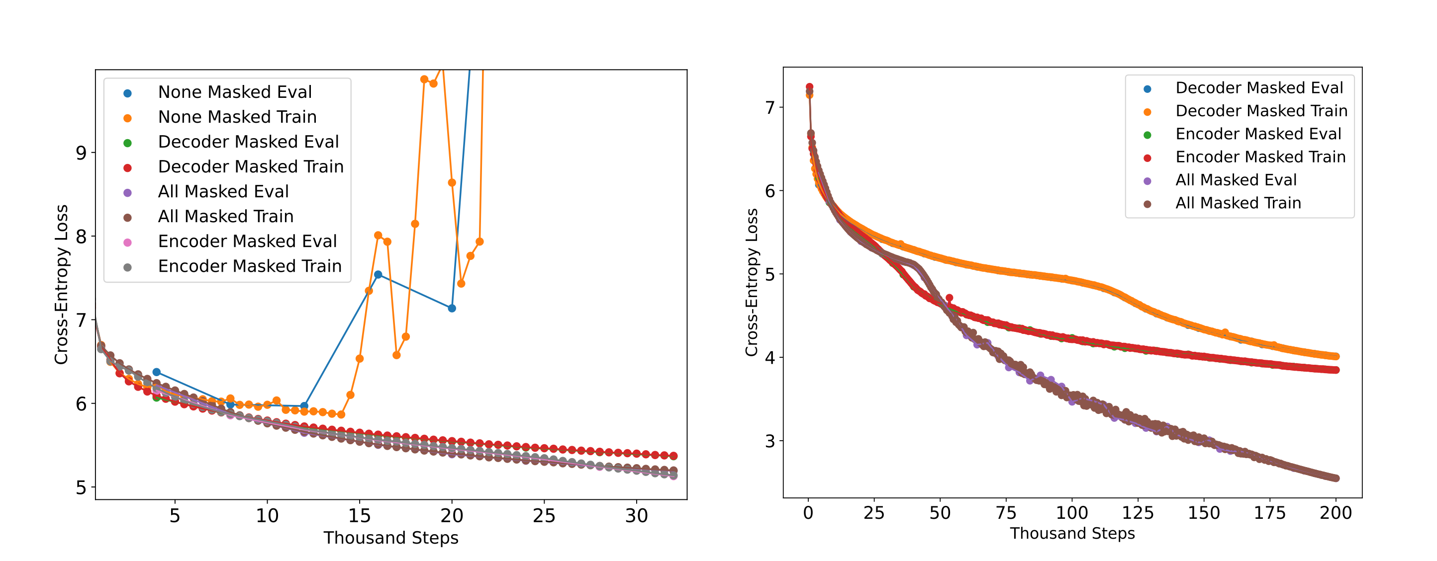
Why would causal masking be so important to a model that does not perform causal modeling? There is usually some benefit to matching a model’s structure to any prior we know about the dataset that is being modeled, and with that perspective one could perhaps guess that enforcing causality is beneficial because the data being modeled (text) is in some way fundamentally causal as it is understood in one orientation. It is less certain why removing all causality masks leads to highly unstable training, as one may expect for a simple decrease in efficiency in this paradigm rather than exploding gradients.

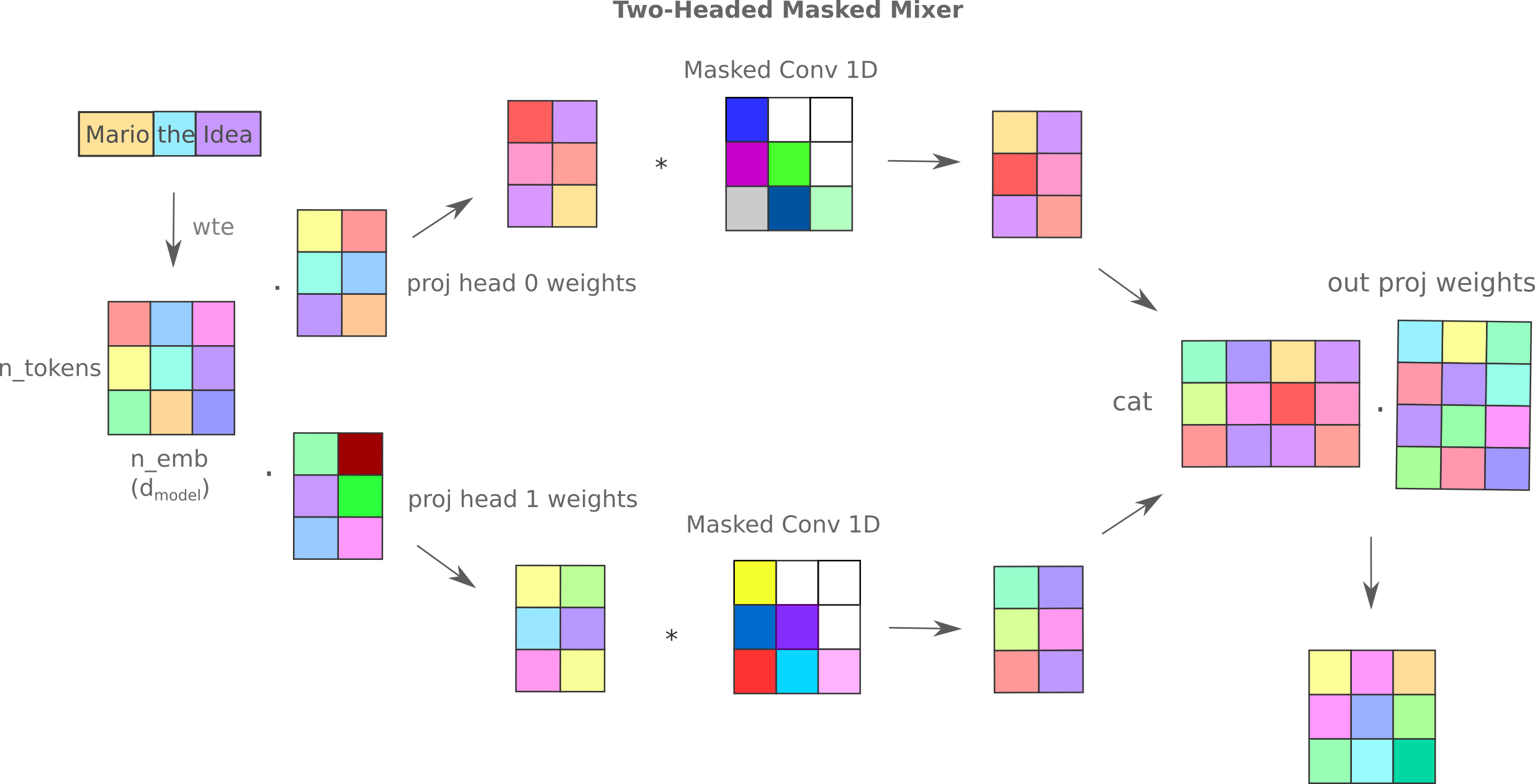
Multi-headed mixer autoencoders

If the mixer is a better autoencoder encoder and decoder in this paradigm (where we regenerate all tokens of a sequence in one pass), how might one improve the mixer’s architecture for further training efficiency? One straightforward guess might be to increase the number of inter-token trainable parameters, and this increase may be achieved in a number of different ways (multiple convolutional kernels, expanded convolutions with nonlinearities, multi-headed masked mixers) but when a number of architectures were tested for causal language modeling the most performant among these was the multi-headed mixer. The linear algebraic transformations that occur in the multi-headed mixer for the case where we have $n_h=2$ heads and the total projection dim is greater than the hidden dimension may be illustrated as follows:

We modify the original multi-headed mixer architecture for the case where there are $n_h=2$ heads and the projection dim is just $d_m / n_h$, and fix $n_l=8$ for both encoder and decoder, and replace the mixer autoencoder’s masked convolutions with these multi-headed convolutions.

As long as we stick to the $d_m / n_h$ total projection dimension limitation, the number of inter-token parameters $p$ for a model with $n_l$ layers and $n_{ctx}$ context is

\[p = n_l (n_h * n_{ctx}^2 + 2d_m^2)\]

whereas we have $p = n_l * n_{ctx}^2$ inter-token parameters for the ‘flat’ masked mixer. Therefore we have a linear increase in inter-token parameters as the number of heads in this scenario, with a constant factor for the addition of any head. To see how to arrive at this number, observe that each head has a corresponding convolution (with weight matrix of size $n_{ctx}^2$) and the input and output projections are unchanged as the number of heads increases, in particular the output projection is size $d_m^2$ and the input $d_m*d_m *n_h / n_h$, and each head contains one 1D convolution.

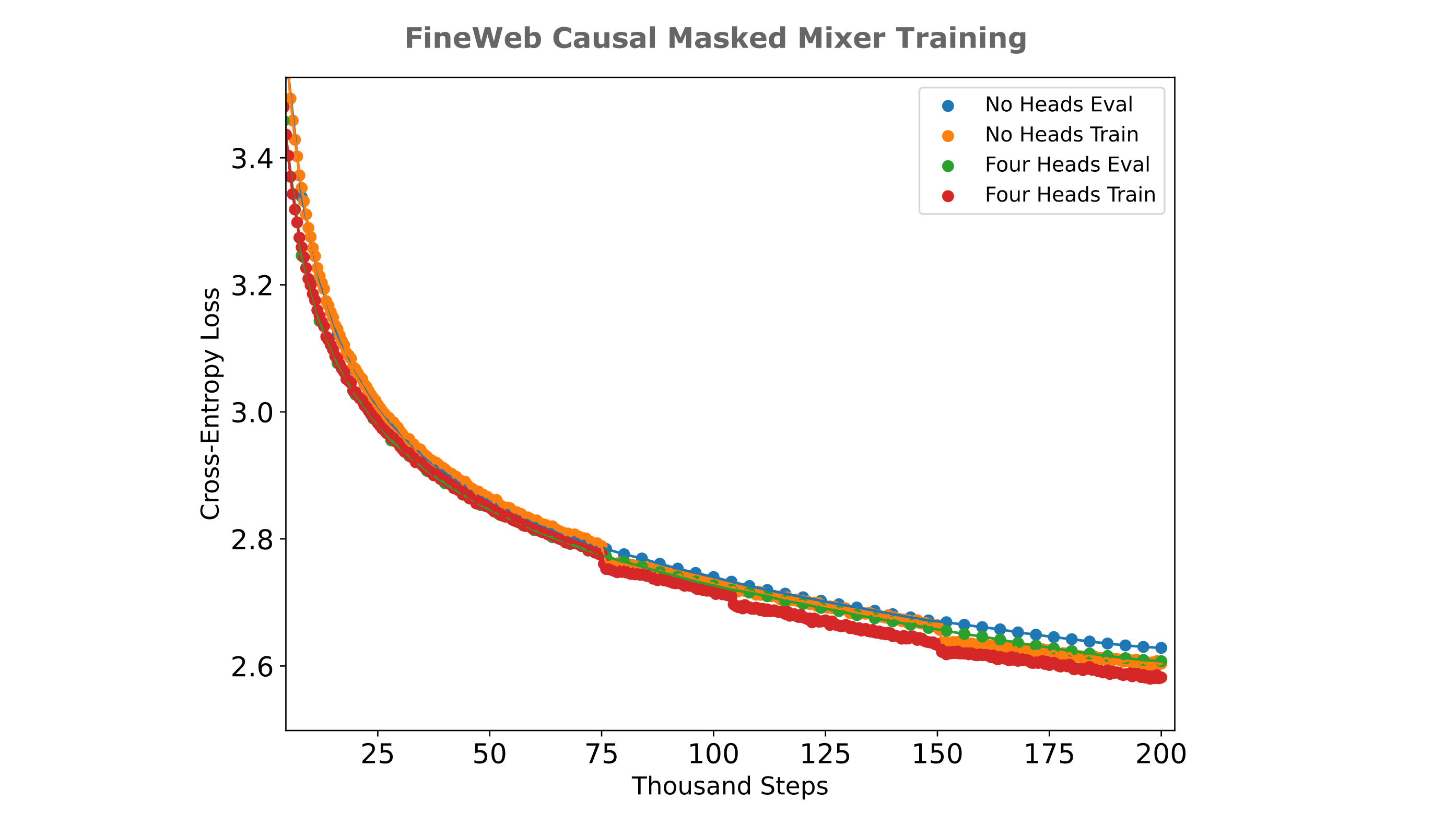
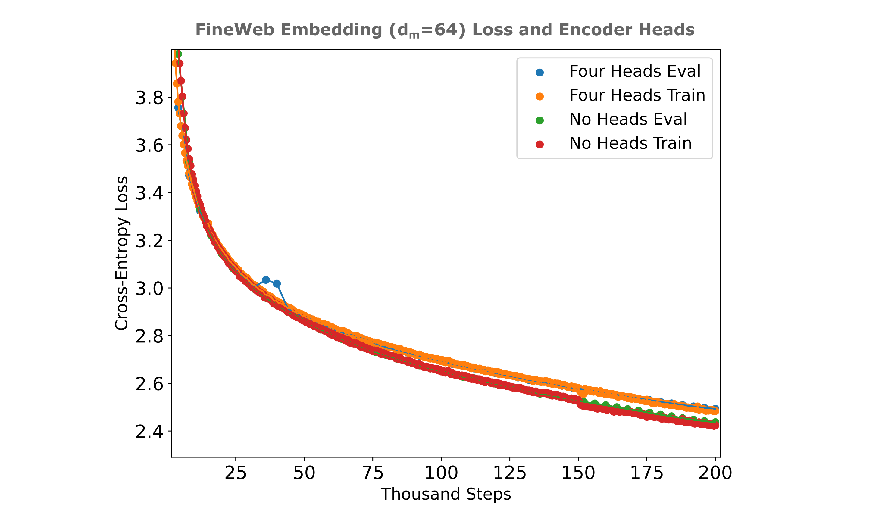
For the case where we keep the concatenated projection dimension to be equal to $d_m$ as above, we have a notable increase in autoencoder training efficiency (see the figure below) relative to the ‘flat’ masked mixer which has no projections and only a single 1D-convolution. From the results below, it is clear that increasing the number of heads leads to greater training efficiency, and the gap between autoencoders with four or more heads and the flat masked mixer architecture is substantial.

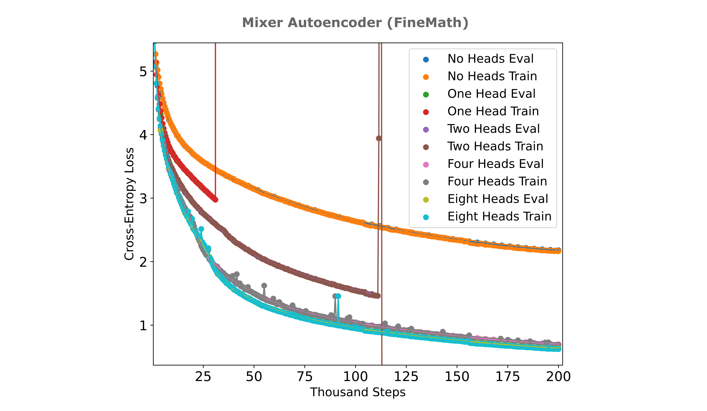
From the figure above one clearly reaches limited returns when expanding beyond four heads as there is a significant computational burden but very little efficiency benefit with an increase to 8 heads from 4, and an efficiency detriment if we increase to 16 heads from 8. It is curious that four heads are also optimal for causal transformer models of similar size with respect to loss achieved per unit of compute applied during training for this dataset as well.

Interestingly, however, the multi-headed mixer autoencoder experiences instabilities late in training manifesting in very rapidly exploding gradients for models with one or two heads. As this was observed early in training for autoencoders without causal masks, one straightforward explanation would be a problem with the multi-headed mixer’s masks. We causally mask the convolution in each head, and a quick test shows that the encoder and decoder modules are indeed causal. A relatively straighforward solution for this problem would be to add a layer or RMS normalization to the concatenated projections, or add residuals across head elements. We can avoid these architectural changes by carefully choosing a datataype, however, as explained below.

A straightforward way to address gradient overflow is to use a datatype with a wider dynamic range than fp16 (which is by definition e5m11), for example either fp32 (e8m23) or the nearly equivalently expressive bf16 (e8m7). bf16 is supported on newer hardware (A100s and H100s and RTX 30 series and above, and although it can be emulated with V100s this emulation cannot make use of the tensor cores in that GPU and is thus low-throughput) and is well supported for bf16/fp32 mixed precision training integration by Pytorch. When we train the same models using bf16/fp32 precision, we no longer observe catastrophic instabilities in multi-headed autoencoder trainings (see the above figure for an example) which supports the hypothesis that numerical overflow is the cause of training instabilities in multi-headed mixer autoencoders.

There is a substantial decrease in loss per step for causal autoencoders trained on the FineWeb as well, although we also find exploding gradients leading to a catastrophic increase in training loss for multi-headed mixer autoencoders. As the exploding gradient and loss problem appears pervasive for multi-headed masked mixer autoencoders, one can attempt to understand why this is the case. A good first candidate could be the datatype we are using for training which is fp16/fp32 mixed precision to allow for older hardware (V100) compatibility. Although this training is usually decently stable across a wide range of model, one can argue that an autoencoder of this type is inherently unstable with respect to gradient norms as all gradients flow through one vector, which is susceptible to numerical overlfow if the vector’s partial derivatives are sufficiently large.

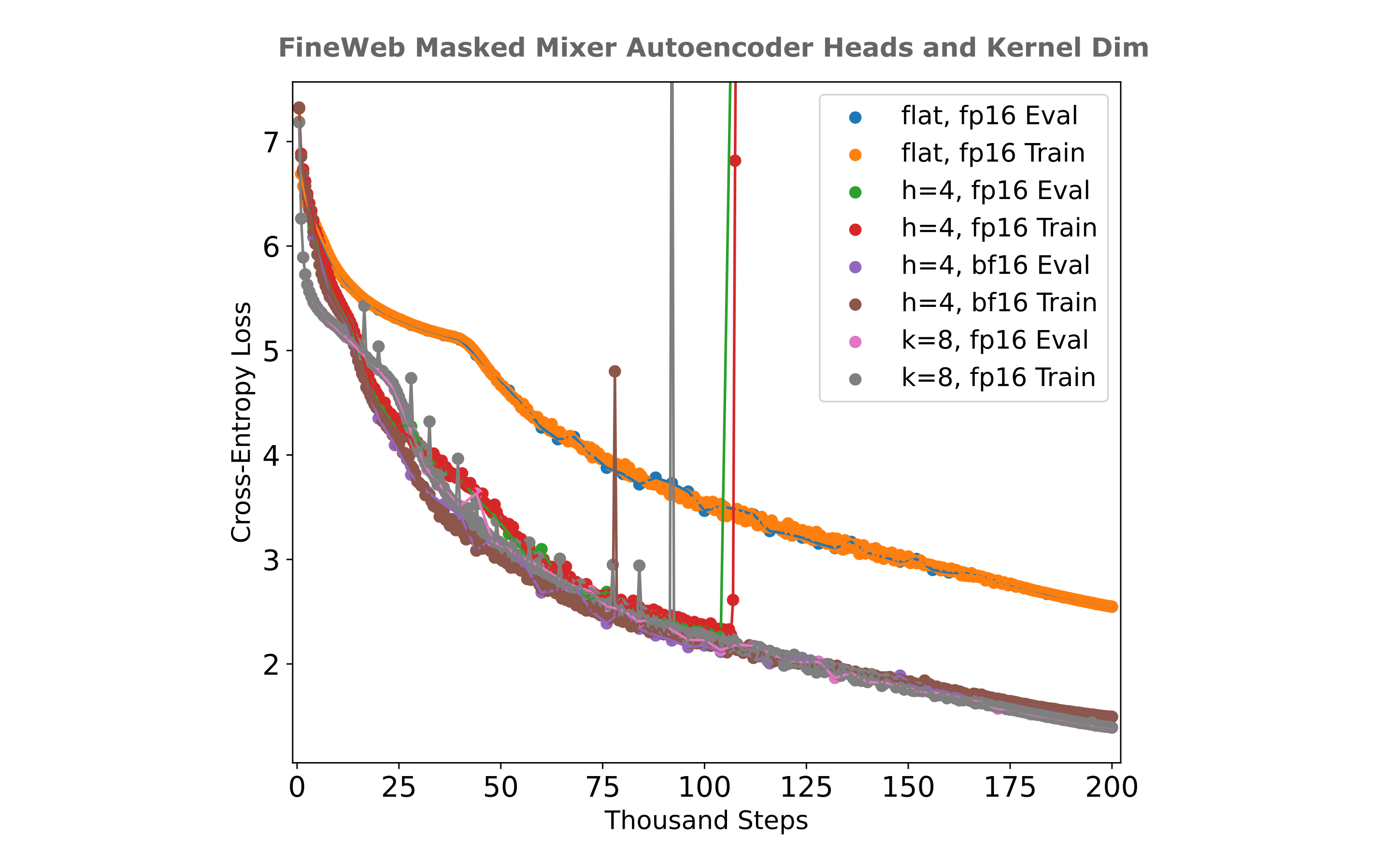
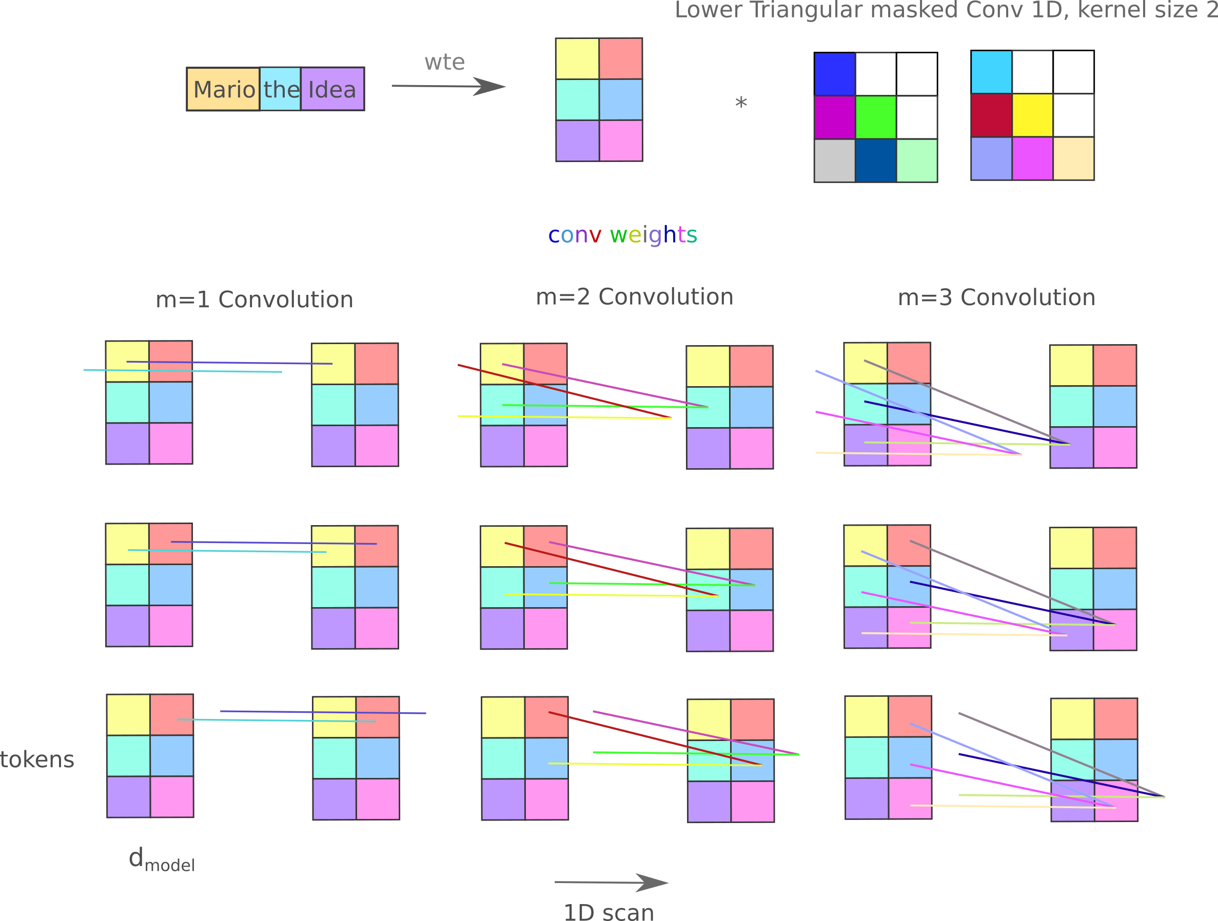
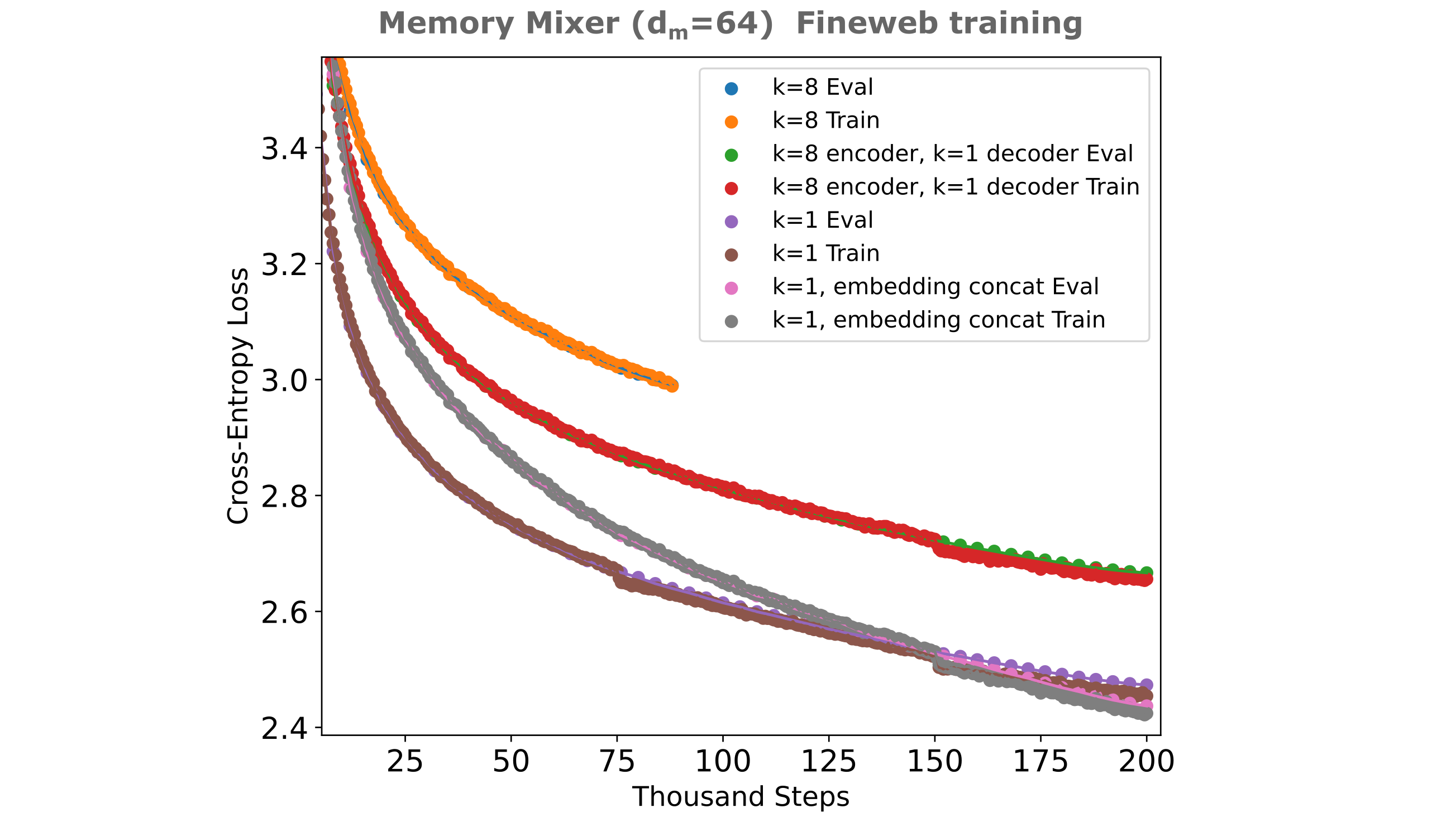
One can increase the number of trainable inter-token parameters in a simpler way than using multiple heads: using a convolutional kernel of size greater than unity (k=2 here denotes two kernels) scales the number of inter-token parameters as

\[p=n_l (k * n_{ctx}^2)\]

as there are simply $k$ weight maps per convolutional layer. From the figure above it is apparent that a flat masked mixer with k=8 achieves identical loss to the 4-headed mixer, but does not suffer the numerical instabilities associated with the latter. For clarity, a figure depicting how a $k=2, n_{ctx}=3, d_m=2$ layer operates is provided below: note here that kernels $k>1$ convolve not only across one hidden layer’s embedding index at a time as $k=1$ mixers do, but contain inter-token embedding parameters such that convolutional weights are trained where a token’s embedding element at position $n$ affects all other token’s embedding elements (causally, that is) at positions $\lvert n - p \rvert < k$. Effectively we have both inter-token and intra-token weights in one layer when $k>1$.

It is also noteworthy that there is such a large difference in training efficiencies for multi-headed versus flat masked mixers for autoencoders. One can estimate the increase in training efficiency by finding the number of samples required to reach a certain loss value, and in this case one requires more than 6x the number of samples for the flat masked mixer to approach the loss achieved by the 4- or 8-headed autoencoder at 200k steps. For comparison, the difference in causal language model loss per step between flat and multi-headed mixers is very small: the flat mixer requires only around 1.05x the number of samples to match the 4-headed mixer when trained on TinyStories. If we implement a causal masked mixer while keeping the projection dimension equal to $d_m/n_h$, we find that there is very little difference in per-step loss between this model and the flat masked mixer when trained on the FineWeb-edu (10BT) dataset.

Text Compression Background

Although it may not seem to be very important to the field of artificial intelligence, text compression in many ways has been proven time and time again to be a very apt predictor of a language model’s abilities across the spectrum and has been shown to be important for everything from language generation to q/a chat capability to chain-of-thought reasoning capability.

Language compression is an old goal, and attempts to understand how to compress text and how much text can be compressed go back to the beginnings of information theory. Shannon’s seminal work focuses on the problem of compression and transmission of textual information, as does earlier work in the field from Hartley and Nyquist. There were practical reasons for that: it has long been appreciated that one needs to send much less information to regenerate a string of characters than to generate the sound of someone speaking those characters, so figuring out exactly how much information is required was and is an important problem to data transmission.

We focus on compression rather than transmission, although one can view deep learning models themselves as being somewhat similar to noisy communication channels. One of the most general methods of measuring text compression is bits per byte (bpb), which is the number of bits required for encoding a byte of input text. Often the input is assumed to be encoded in UTF-8, which uses one byte per character and makes this measure effectively the number of bits per input character if single-byte encoding predominates.

Although less well known than other model capabilities, the most effective text compression methods today are frontier large language models trained to predict each next token in a very large corpus of text. The gap between classical compression algorithms and these models is vast in the scale of information theory: perhaps the most widely used compression algorithm gzip achieves up to around 2 bits per byte, highly tuned dictionary and bit matcher decoders achieve around 1.2 bits per byte, whereas Deepseek v3 achieves 0.54 bits per byte.

The way large language models are usually used to compress text is simply by being able to predict next tokens, where the compression is simply the number of bits required to correct errors in the model’s prediction for each token. Causal language model-style compression is nearly as old as text compression itself. For example, Shannon used next character prediction by people as a way to attempt to estimate the source entropy for the English language. Shannon estimated a lower bound of around 0.6 bits per character, very similar to what we see for large language models today.

There is a clear upper bound to causal language model text compression, however: in natural languages such as English, there is a certain amount of inherent ambiguity such that no particular word necessarily follows from a given previous sequence of words. This is what Shannon referred to as ‘source entropy’, and it may be thought of as irreducible error and provides a hard lower bound on the bits-per-byte compression of a causal-style model.

With this in mind, we have a clear alternative to next token prediction-based compression. We can use our new masked mixer-based autoencoder to compress the input directly and thereby avoid the problem of source entropy alltogether. The reason for this is that our autoencoder effectively compresses the entire input into one vector and uses this vector to reconstruct that input, where the source entropy becomes irrelevant for an arbitrarily powerful autoencoder capable of capturing all necessary information in the embedding vector. In real-world applications the source entropy is clearly important to the ease of actually training a model (as we shall see for mathematical versus general text later), but in the idealized scenario of arbitrary power our only lower bound is the size of the autoencoder’s embedding.

Text Compression via Autoencoders

If we have a negative log likelihood loss $\Bbb L$, we can compute the number of bits per input byte for a given segment of text if we know the length of text in bytes $L_b$ and the number of tokens required to encode that text for a given tokenizer $L_t$.

\[\mathtt{BPB} = (L_t / L_b) * \Bbb L / \ln (2)\]

On this page we report loss as the torch implementation of CrossEntropyLoss, which is equivalent to taking the Negative Log Likelihood of a softmax-tranformed logit output. This means that we can simply substitute our CEL loss values for the negative log likelihood $\Bbb L$ values (the softmax simply transforms the model’s outputs to a probability distribution). We also make the simplifying assumption that our text is encoded in single-byte UTF-8.

We can now compare the compression achieved using masked mixer autoencoders to that obtained when using next-token-prediction models. Taking the FineMath 4+ dataset and a tokenizer that averages 2.82 characters (which equals 2.82 bytes assuming single UTF-8) and a model with a 512-dimensional embedding with an $n_{ctx}=512$ stored using 4 bits per parameter, we can calculate the amortized BPB as follows:

\[\mathtt{BPB} = \frac{n_p * b_p}{n_{ctx} * (L_b / L_t)} \\ \mathtt{BPB} = \frac{512 * 4}{512 * 2.82} \approx 1.42\]

assuming that we have zero loss after training (we actually have around $\Bbb L=0.7$). This compares disfavorably with the compression achieved by a causal language model transformer on this dataset using approximately the same compute,

\[\mathtt{BPB} = (L_t / L_b) * \Bbb L / \ln (2) \\ \mathtt{BPB} = (1/2.82) * 1.4 / \ln(2) \approx 0.72\]

A straightforward way to attempt to increase the compression in our autoencoder is to use a smaller embedding, perhaps to 128 parameters. In the following figure, we train mixer and transformer-based autoencoders using embeddings of size $128$ on Fineweb using $n_ctx=512$. The 8k-size FineWeb tokenizer averages 3.92 characters per token on that dataset, resulting in the following lower bound for compression using this model:

\[\mathtt{BPB} = \frac{n_p * b_p}{n_{ctx} * (L_b / L_t)} \\ \mathtt{BPB} = \frac{128 * 4}{512 * 3.92} \approx 0.255\]

Unfortunately after 200k steps (which equates to 13 billion tokens, or around 12 hours on a 4x A100 node) these autoencoders are no where close to achieving this compression, as their loss is far from the origin. Somewhat encouraging is the observation that these models do not exhibit exponential decay scaling in terms of loss per number of tokens trained (below right, observe the lack of linearity on the semilog axes), suggesting that if much more compute were to be applied they may be capable of effectively reaching zero loss.

Embedding-augmented causal language models

Recalling our original motivation to introduce input embeddings to remove the source entropy of text for a language model compressor, it may be wondered if one cannot combine the advantages of the autoencoder with next token prediction-based compression. The reson why this might be beneficial is as follows: it is apparent that masked mixer autoencoders require a compressed $d_m$ that is too large (in bits per $n_{ctx}$ tokens) to improve upon the compression found using next token prediction models given the relatively small amount of compute we have been applying to train these models.

The primary reason for this is that each token (which usually represents between 3 and 5 bytes of text) is greatly expanded by the embedding transformation, whereby each token becomes represented by vectors of at least 512 elements, or at least 1024 bytes in fp16. This is such a large expansion that even our subsequent many-to-one token compression abilities do not give greater total compression than causal language models.

Some reflection may convince us that there is a good reason for this: it may be conjectured that our autoencoder is less efficiently trainable than a next-token-prediction model (for our compute) because it must generate the entire context window in one forward pass, whereas the causal language model generates one next token at a time using information from all previous tokens.

With this in mind, it may be wondered if we can combine the advantages of causal modeling and autoencoding to make an encoder-decoder architecture that exhibits superior compression ability to either autoencoder or causal language model alone, give similar compute to what has been used previously.

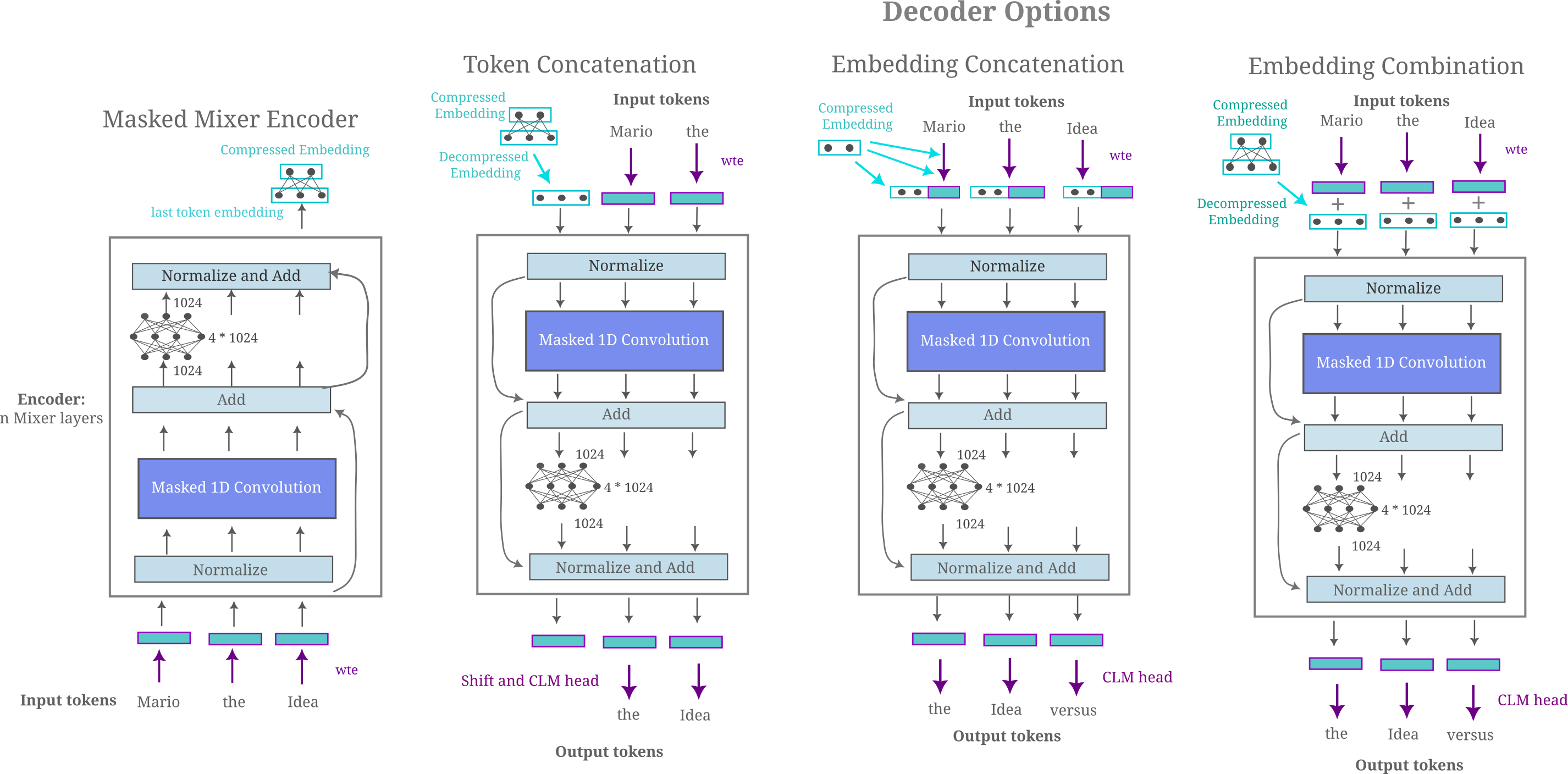
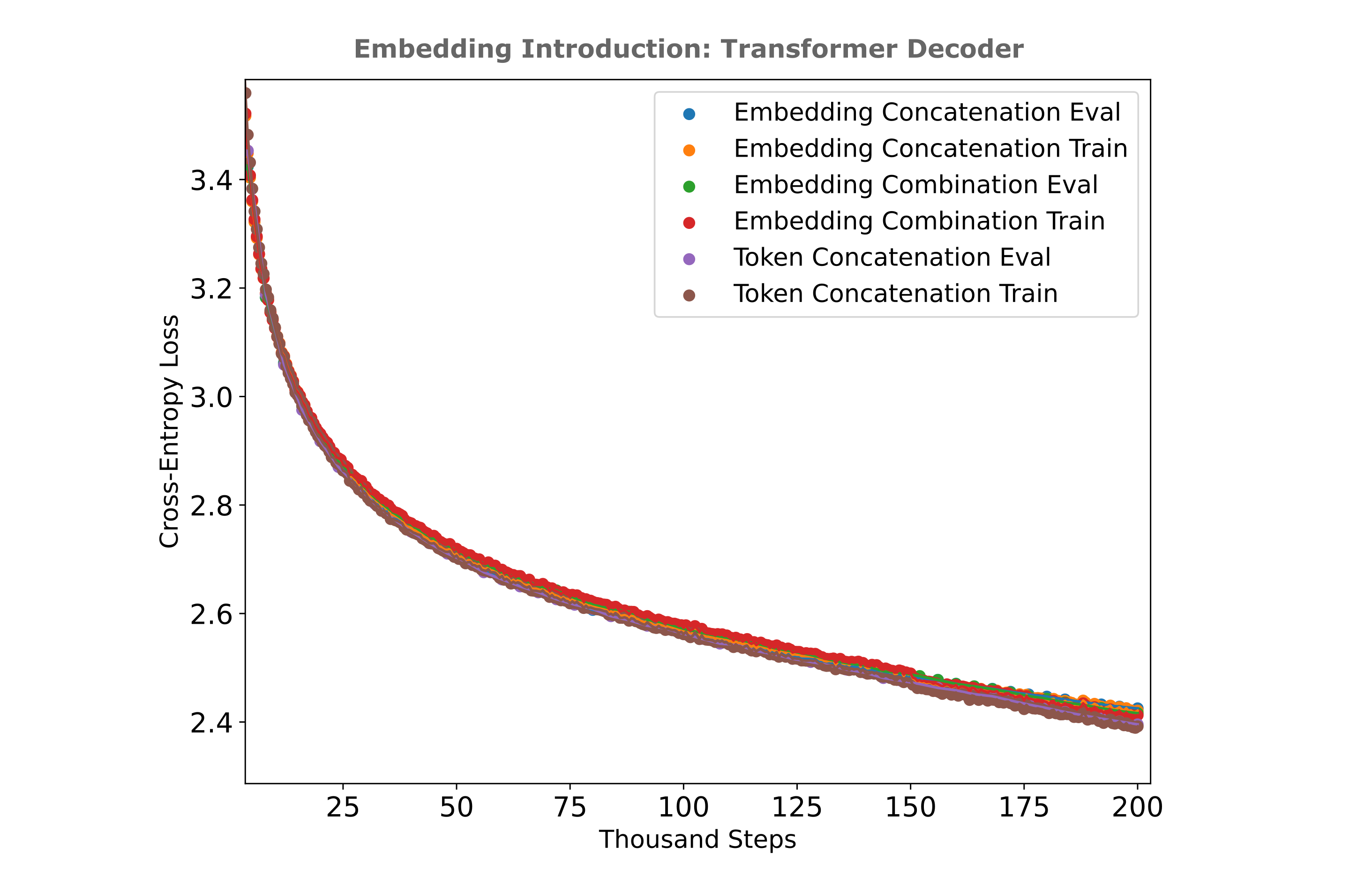
There are a number of options for how one could introduce the encoder’s embedding into the decoder. Three straightforward candidates are concatenation in the token dimension, concatenation in the embedding dimension, or a linear combination in the embedding dimension. For embedding concatenation, we decrease the size of the token embeddings for the decoder commensurately to maintain a constant decoder size while comparing to other methods. These are illustrated in the following figure for convience.

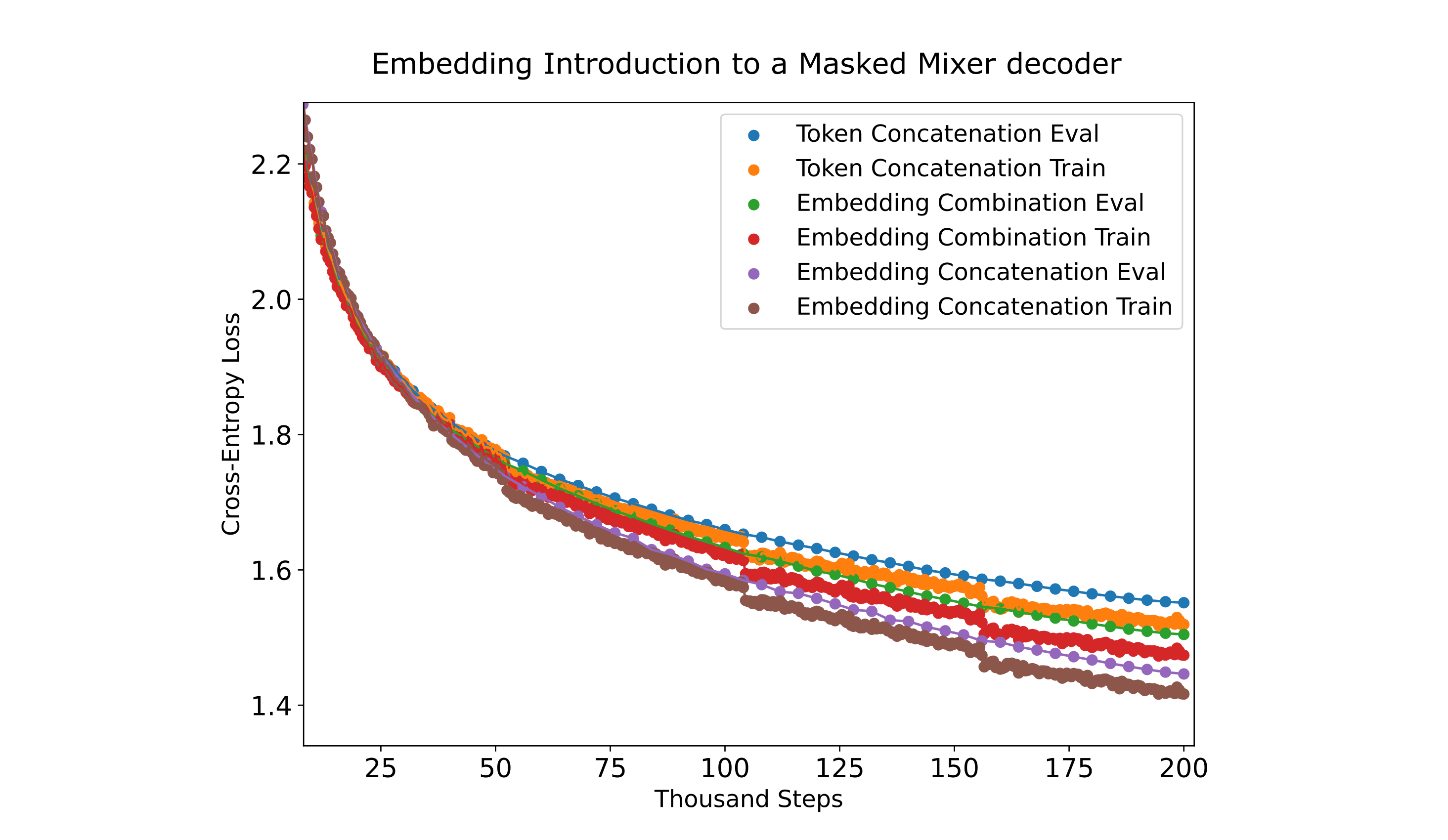
When we test the use of these three methods on FineMath 4+ data using a masked mixer decoder as our causal language model, we find that in general they are similarly efficient to train with the embedding concatenation method obtaining a slightly lower loss than embeddings combination or token concatenation.

One may expect for a transformer decoder to exhibit more training efficiency if given a token concatenation relative to embedding concatenation or combination, and indeed this is what we find (this time applied to the FineWeb-edu dataset):

It appears from the above results that transformers are relatively invariant to how exactly the encoder’s embedding is introduced among these three methods, so for text compression purposes we will use them interchangeably.

Can adding an encoder’s embedding lead to increased compression? To answer this we first need to know how large our embeddings are (particularly how many bytes they require) and then we can convert this to a bits-per-byte value. Suppose one trains an embedding-augmented causal model where the embedding is of dimension $n_p$, each parameter being stored using $b_p$ bits, for a context window of size $n_{ctx}$ and $L_b / L_t$ bytes of input text per token. Then we can calculate the bits per byte required to store this embedding (amortized over the input) as previously via

\[\mathtt{BPB} = \frac{n_p * b_p}{n_{ctx} * (L_b / L_t)}\]

Once this value is known, we can find the loss offset $\Bbb L_o$ that corresponds to this extra required information,

\[\Bbb L_o = \frac{\mathtt{BPB} * \ln (2)}{(L_t / L_b)}\]

and add this offset to the causal language modeling negative log likelihood loss for next token prediction to find the total loss.

\[\Bbb L = \Bbb L(O(a, \theta), y) + \Bbb L_o\]

We call this the ‘normalized loss’ for brevity. For a relatively small embedding ($d_m=64$) assuming 4 bits per parameter, and with a context window of $n_{ctx}=1024$ we have the following normalized loss (all masked mixers in the following figure are flat, and all models except the transformer->transformer use embedding concatenation introduction which uses token concatenation introduction):

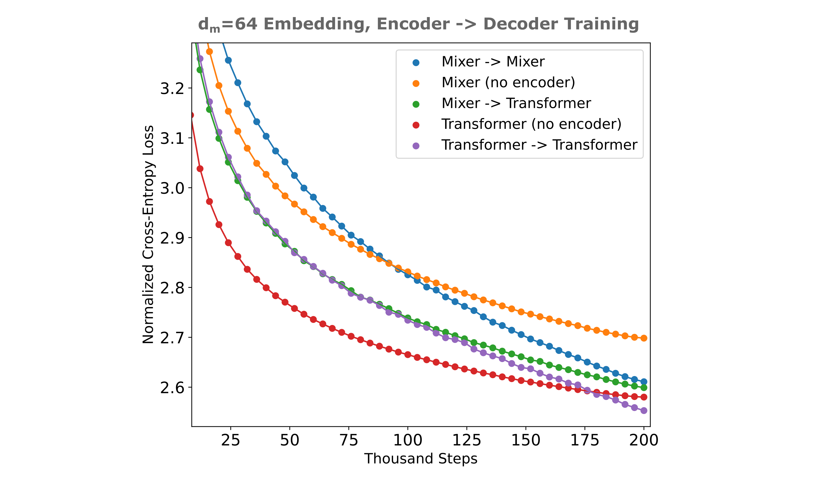
There is some expected behavior here: the embedding-augmented models begin training with higher loss (the result of the offset required for storage of the 64 floats in the embedding vector) but then approach or pass the purely causal model’s loss (or equivalently its bpb compression of the input). We can see this most clearly by observing the difference between embedding-augmented and plain causal model at a given step or causal model loss value as shown in the following figure. As we expect for the embedding to allow a model to circumvent the difficulty of learning a corpus with a certain amount of language-intrinsic source entropy, we would expect for the embedding to be less useful early in training when this source entropy is a small part of the total model’s cross-entropy loss with respect to the text corpus.

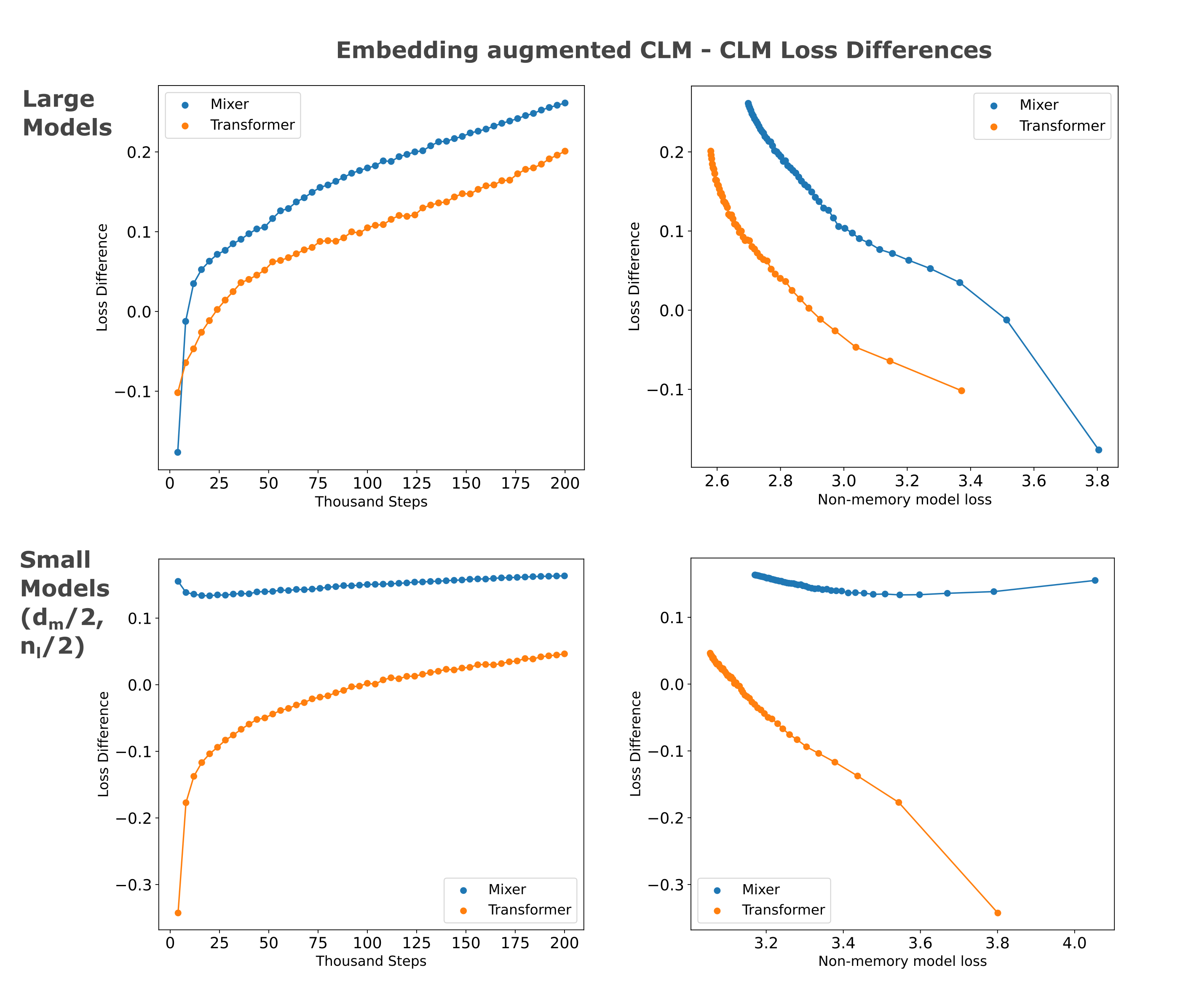
It is somewhat less expected that the masked mixer decoder appears to be able to learn to use the information present in the embedding more efficiently than the transformer decoder, a pattern that is particularly apparent later in training. As the transformer encoder -> transformer decoder model exhibits the same tendancy, this could result from an alignment between encoder and decoder with respect to architecture.

We may wonder whether this near-linear loss decrease for embedding-augmented models persists as models are trained on more tokens. We find that this is indeed the case: training on more samples (with the same lr scheduler and batch size etc.) leads to the masked mixer achieving the lowest total bits per byte, assuming 4 bits per parameter for the embedding. Even assuming that one can only quantize the embedding to 8 bits per parameter, we find that the memory transformer exceeds the compression of the causal-trained transformer on this dataset.

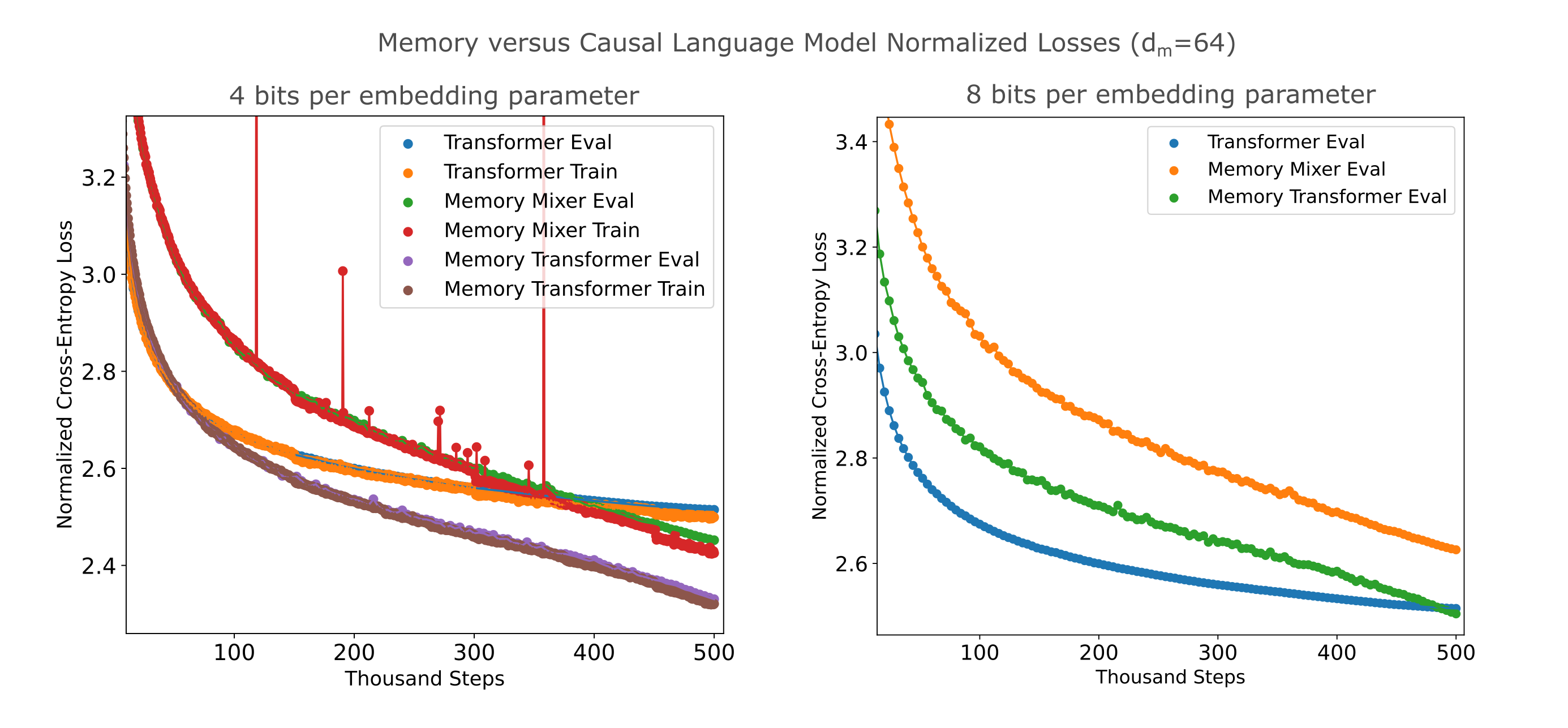
From these results it appears that the informational content of the embedding (only 64 parameters in this case) is not saturated even after a relatively long training run such that the loss continues to decrease nearly linearly. It seems safe to assume that the embedding-augmented mixer would be a more efficient compression model for a fixed compute applied at training even if the embedding were quantized with 8 or 16 bits per parameter.

The above results are obtained for flat masked mixers, and as we observed superior training efficiencies with multi-headed mixers of the same size one may expect to find better training properties for embedding-augmented causal mixers as well. It comes a some suprise, therefore, that an embedding-augmented causal masked mixer (using embedding dimension concatentation) with four-headed mixer layers in the encoder slightly underperforms the same model without heads as shown in the figure below. Note here that $d_m=64$ denotes the embedding dimension, where use use a 256-width encoder and 1024-width decoder.

A similar result is obtained where we instead increase the number of inter-token parameters by using convolutional kernels of size four rather than one, where we see no increase in training efficiency upon doing so when the encoder’s embedding is introduced via embedding concatenation but curiously not when we use token dimension introduction for the embedding, in which case there is a notable improvement in training efficiency.

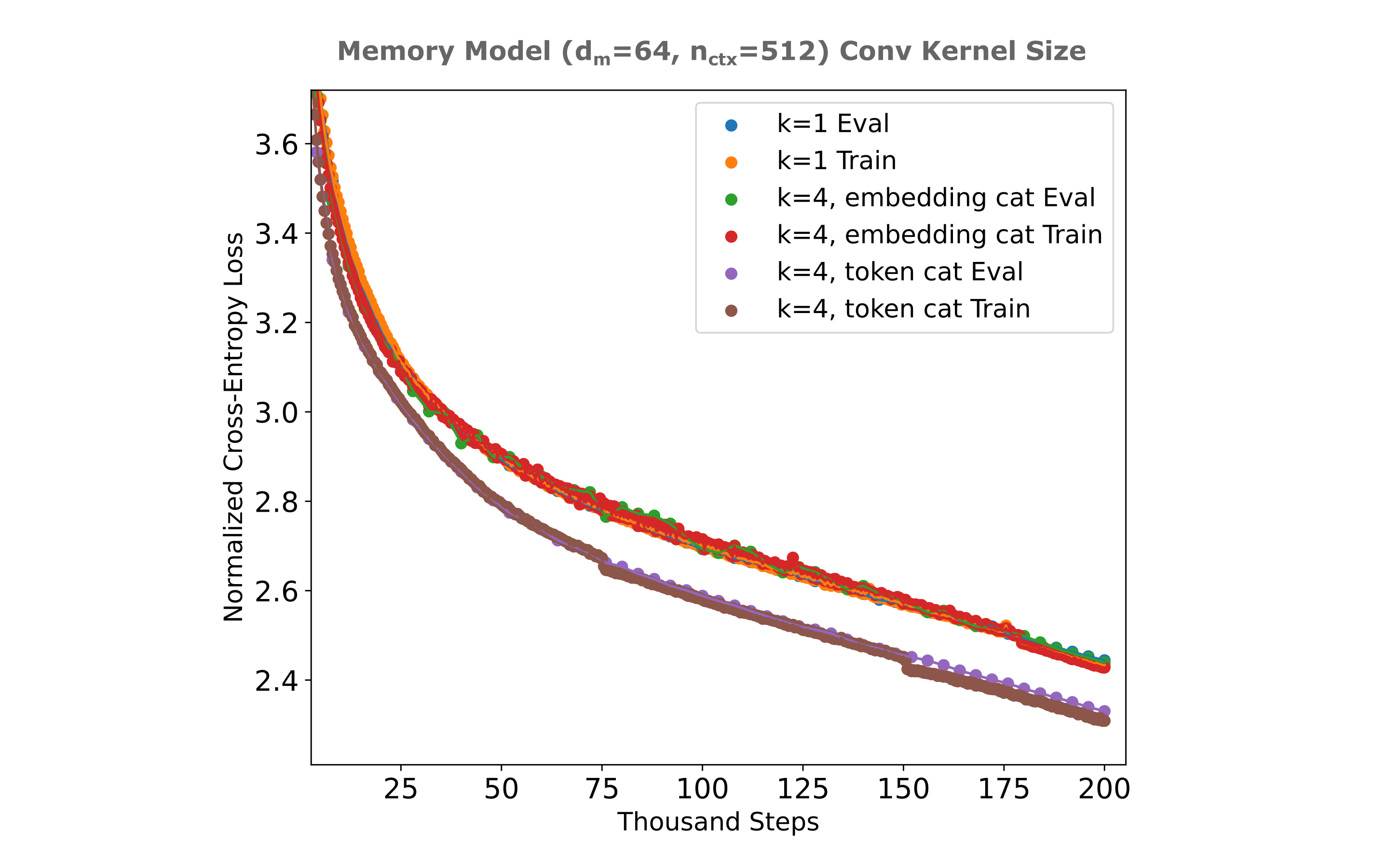
But when we measure the ability of embedding-augmented masked mixers to compress FineWeb at a larger $n_{ctx}=1024$, we see that the multi-kernel mixer training actually exhibits decreased per-step loss relative to single-kernel mixers. As for FineMath, we again observe embedding concatenation to yield slightly more efficient training after 200k steps (~13 billion tokens).

It should perhaps be noted that the dataset we use to train and evaluate tokenizes documents individually and pads if necessary, meaning that not all samples contain the full 1024 token context window of non-pad tokens. This makes our calculation of the amortized bits per byte from the embedding somewhat inaccurate, as that assumed full context in every sample. The reason this is important is because one would expect for smaller-context samples to exhibit lower loss for entropy models if the embeddings of those models were to be capable of retaining a constant amount of information regardless of the number of non-pad tokens present in the input.

We can filter evaluation for only full-context samples for both entropy estimation and causal language models, and doing so yields the following Cross-Entropy Losses:

	200k Entropy	500k Entropy	200k CLM	500k CLM
All Samples	2.379	2.1566	2.5801	2.515
Full Context	2.502	2.2968	2.6121	2.5492

As expected, there is higher loss for entropy estimation models when applied to full-context inputs compared to all inputs, although this is also the case for causal models to a lesser extent. This is a relatively small loss difference, however, and is nearly constant per model over 300k training steps.

We can also observe the cross-entropy losses of entropy estimation and causal language models when all inputs contain the full context window (here $n_{ctx}=1024$) of non-pad tokens, which can be done by packing tokens from various documents into each context window as necessary. In this case, each sample contains tokens from one or more (possibly several) documents concatenated into one sequence, and again we use the FineWeb as our data source. After training an encoder-decoder entropy estimation model and causal model on this dataset, we find a hearly identical difference in losses as the full-context loss above: the entropy estimation model reaches a CEL of 2.535 compared to 2.642 for the causal model at 200k training steps (7 billion tokens).

Embedding Quantization

In the section above, we assumed an 8 bit per parameter quantization would be possible with minimal loss. Is this a reasonable assumption?

There are typically two ways one can take to quantize a model: either train the model using the quantization (or a facsimile of that quantization) which is called quantization-aware training or else train the model in full accuracy (here fp16/fp32 mixed precision) and quantize after training, which is known as post-training quantization. In this case, all we care about is quantizing the activations of one particular layer (activations between the down and up compression transformations) rather than the weights and activations, making this a somewhat atypical quantization investigation. We start by observing post-training quantization accuracy.

Perhaps the simplest post-training quantization we can perform is to cast the activations in our compressed representation layer to the desired data type, assuming that both data types are floating points. There are two pytorch-native 8-bit floating point data types: float8_e5m2 (five bits for the exponent, two for the mantissa, and one for the sign) and float8_e4m3fn (four exponent, three mantissa, and one sign bit and one bit pattern for NaN overflows), which were originally introduced in this paper. The difference between these data types is effectively more precision for e4m3 versus more range for e5m2.

Embedding Datatype	Loss
Float16 (E5M10)	2.26
Float16 (E8M7)	2.28
Float8 (E4M3fn)	4.86
Float8 (E5M2)	6.65

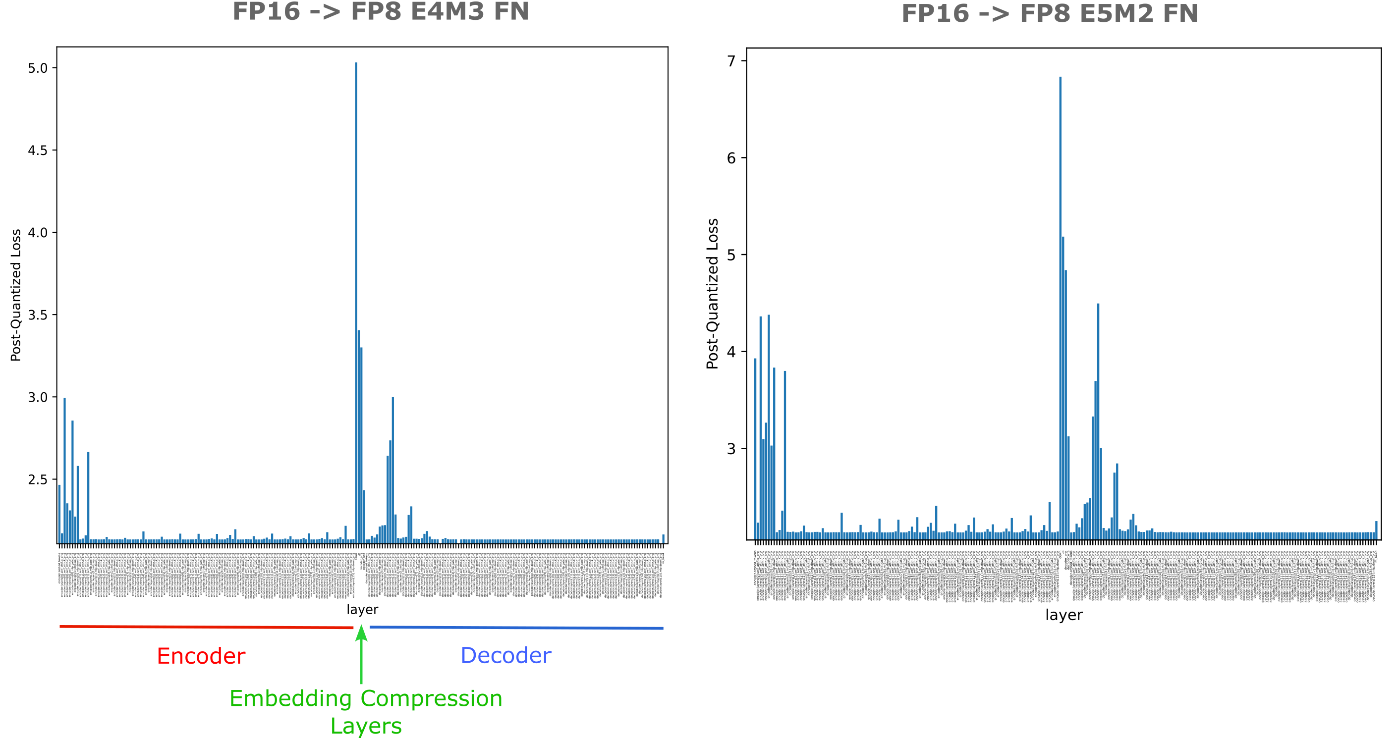
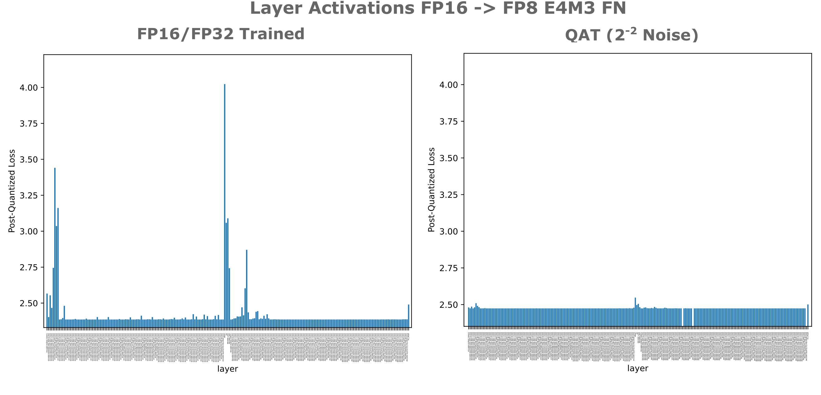
Thus we have a large increase in evaluation loss when we go from seven precision bits to three. This is somewhat surprising given that we are performing relatively mild quantization on activations of only one layer. It may be wondered whether this is typical of layers in oracle memory models or not, and we can investigate this question by performing quantization on the output activations of each linear transformation in our model, observing the resulting evaluation loss with each quantized layer. In the folling figure, we see that indeed the activations of down and up projections are by a wide margin the most sensitive of all layers in the model.

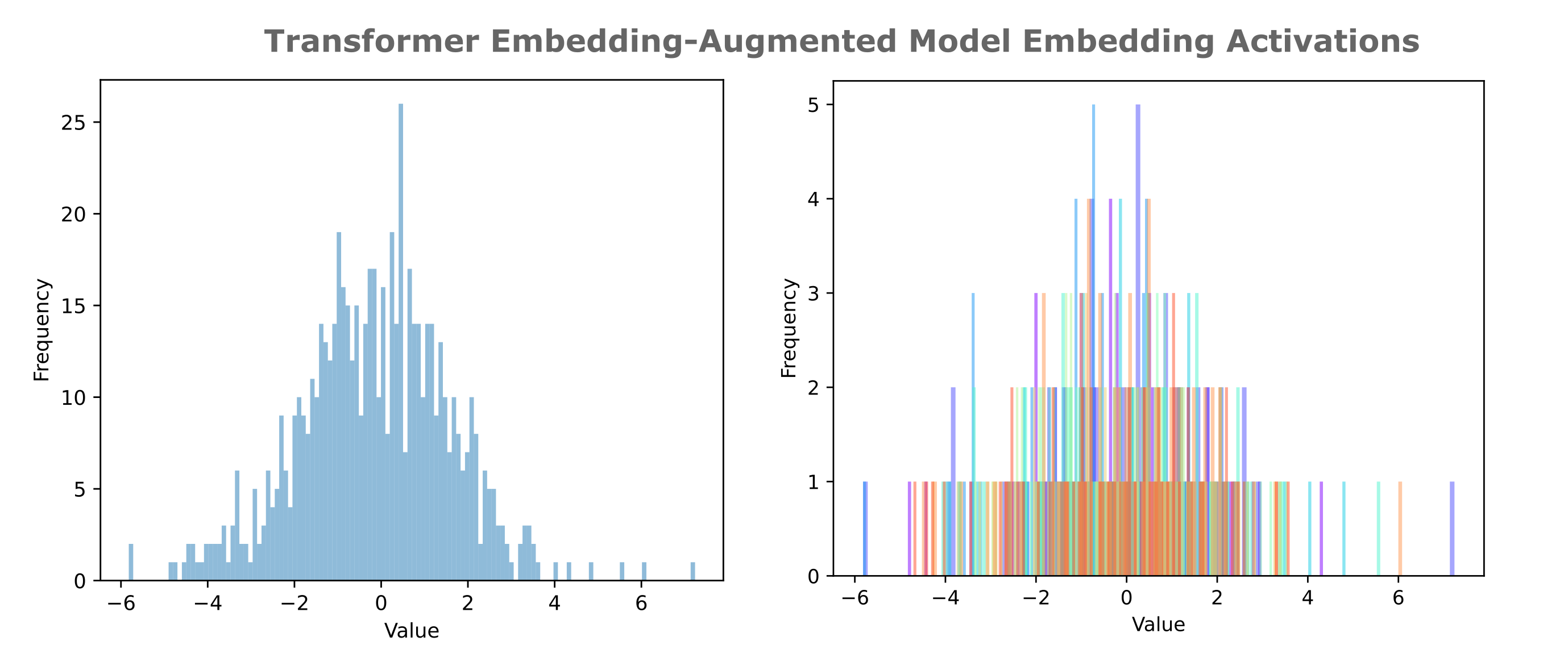
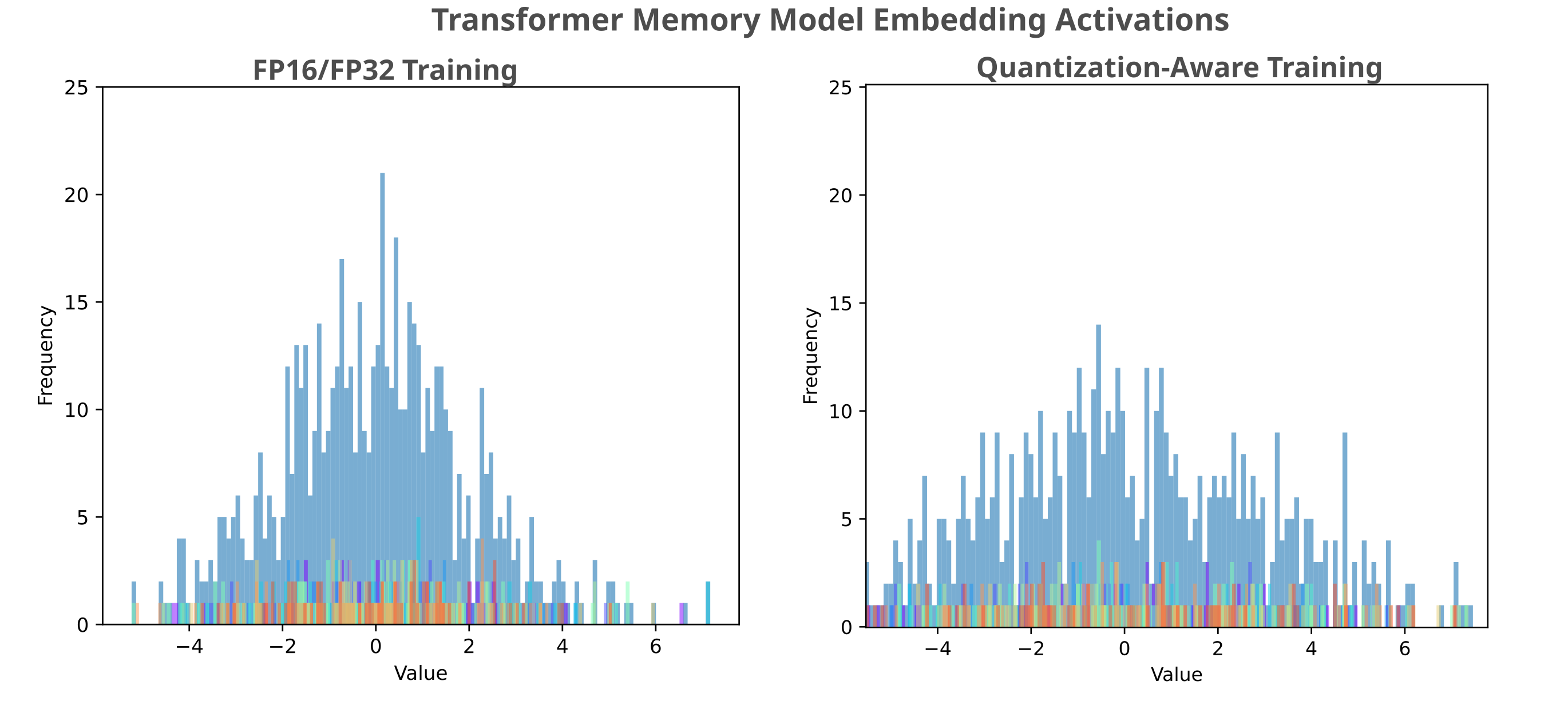
When we observe the distribution of activations typical in this embedding layer, we see the reason: activations for ten samples divided into 128 buckets (the most represntable by 8 bits) lie entirely within [-7, 7] and thus we only require three bits in the mantissa, but there is substantial overlap in activation values given this bucket size near the origin. In the following figure, we observe the distribution embedding activation values for ten samples, aggregated on the left and separated by color (ie all red bars correspond to activations from one sample). The right panel shows that there generally not a distinct drift in mean and variance between samples.

A more sophisticated quantization approach is to use the statistics of the distribution of activations to attempt to assign buckets (quantized values) such that the probability of two distinct values becoming quantized to the same value is minimized. From the above figure it appears that our data follows an approximately normal distribution, which is typical of language model activations. One successful approach to near-lossless quantization of such values is the Bitsandbytes Int8 matrix multiplication algorithm in which activations and weights are quantized to 8 bits per element and multiplied and unquantized, with large outlier parameters held out and processed at full precision. We observe little to no large outliers in our activation distribution, and thus can assume that 8 bit quantization is applied to nearly every activation element.

We can apply the Int8() approach while avoiding any loss penalty resulting from quantizing weights in addition to activations as follows: we insert a linear layer ‘probe’ into the model in between the down and up compression transformations, and assign this linear probe to have weights corresponding to the identity matrix such that the input and output of this linear layer are identical, $Px = Ix = x$. As the identity matrix contains all zeros and ones, it may be trivially quantized in 8 bits without precision degradation. We can compare the loss obtained quantizing this probe to the loss obtained quantizing the up layer to observe the relative importance of activation-only versus activation-and-weight quantization.

Embedding Datatype	Loss
Float16 (E5M10)	2.13
BNB Int8() on probe	2.47
BNB Int8() on up	2.52

Int8() is clearly a far more powerful quantization method than naieve casting, but we still have a substantial performance gap present. This model (and indeed this particular embedding layer) is much more sensitive to quantization than a typical causal language model, which would normally see a <2% loss difference upon Int8() quantization from FP16 data.

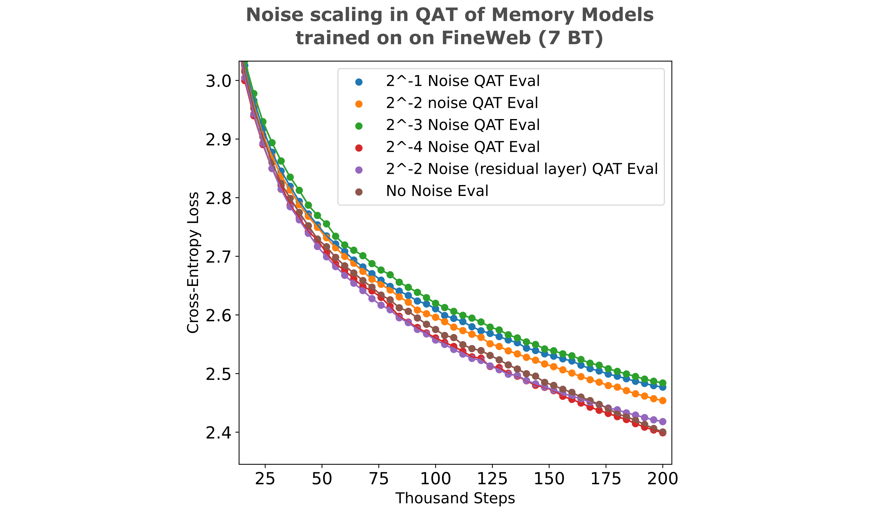
If there is some difficult-to-reduce error upon post-training quantization, the usual strategy is to train a quantization-aware model. We have a particularly simple quantization goal: one layer’s activation quantized to around 8 bits per parameter. As most trainings are performed on older hardware that does not natively support the newer 8 bit datatypesin their tensor cores, we do not actually train using 8 bits per activation but instead use a fascimile of this: we add noise to Float16 activations to approximate the precision achievable using 8 bits, specifically we target the E4M3 datatype with three mantissa bits.

To perform quantization simulation, we add our embedding vector to a vector of identical size of uniform noise scaled to 1/2 the desired precision of $2^{-3}$ (ie x += torch.rand(x.shape) * 2**-4). This makes our down and up operations equivalent to the following where $q=2^{-4}$ and $\mathcal{U}_e(-q, q)$ indicates a vector with the same dimensionality as our compressed embedding $e$ is formed by sampling a uniform distribution bounded by $[-q, q)$,

\[O_{up} = W_{up} \left( W_{down}x + \mathcal{U}_e(-q, q) \right)\]

The use of noise addition to weights to estimate the information required to store those weights is an old trick in the field, and an early use of uniform noise addition to weights in order to estimate the number of bits required to store those weights is found in Sejnowski and Rosenberg. In the linked papers, the authors sought to understand the contribution of each weight (layer) to the model in question by adding noise at various magnitudes and observing the inference accuracy, and the ability to re-train the ‘damaged’ model. In the latter, they estimate the number of bits required per parameter based on this noise amount combined with knowledge of the range of values present. We modify those approaches for quantization-aware training by injecting noise upon each forward pass (rather than only once) in the activation rather than weights and training from scratch, rather than re-training a previously-trained model after one-shot noise addition.

At first glance it might seem strange to add noise to simulate quantization, but doing so simply decreases the effective precision of the embedding vector as given a noised output one can only assign an approximate value. As quantization decreases the effective precision (and range, but that is not as relevant to this implementation) in a similar way, we only have to scale the noise appropriately for the target quantization to achieve near-zero loss gap between noised and quantized implementations. We use a factor of 1/2 the desired quantization precision as the maximum distance any point is away from the closest quantized value is precisely half the distance between quantized values.

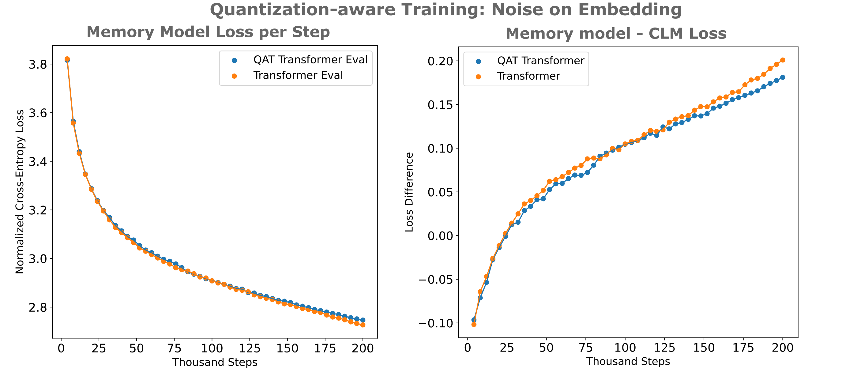
We first note that there is minimal (<0.1%) difference between loss achieved using our noise-added model versus a standard transformer-based embedding-augmented model after 100k training steps, indicating that our noised quantization-aware model trains as efficiently as our unquantization-aware model. When we evaluate this, we observe the following:

Embedding Datatype	Loss
Float16 (E5M10)	2.56
BNB Int8()	2.55
Float8 (E4M3fn)	2.58
Float8 (E5M2)	2.65

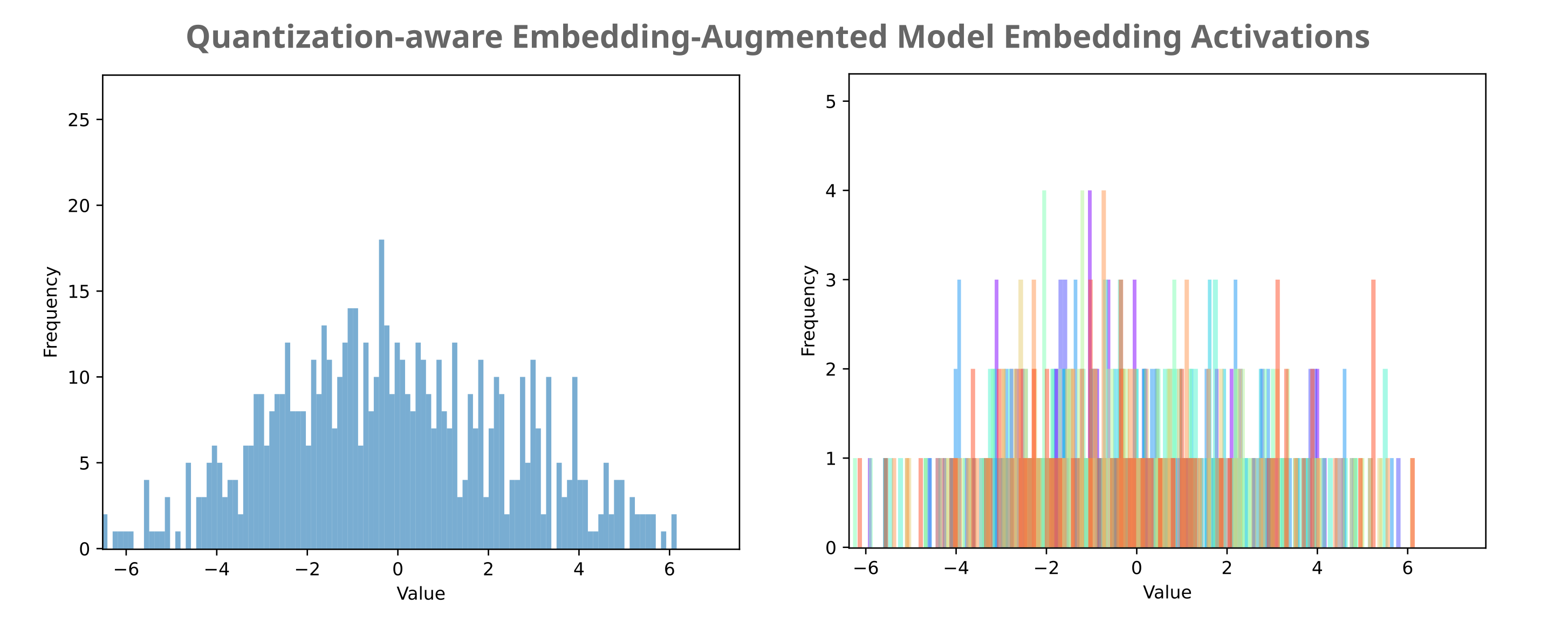
We observe very little loss difference between the unquantized and Float8 E4M3-quantized model, which is what we wanted. We also find no loss decrease upon bitsandbytes Int8() probe quantization, and only a modest loss increase with Float8 E5M2. When we observe the distribution of embedding activations, we find that there is less clustering around the origin but notable we still observe no outliers. We thus expect to be able to quantize to 6 bits per activation using E3M2 with the same amount of loss as E5M2.

After 200k training steps, we have the following:

Embedding Datatype	Loss
Float16 (E5M10)	2.424
BNB Int8()	2.437
Float8 (E4M3fn)	2.672
Float8 (E5M2)	3.253

and the distribution for activations is as follows:

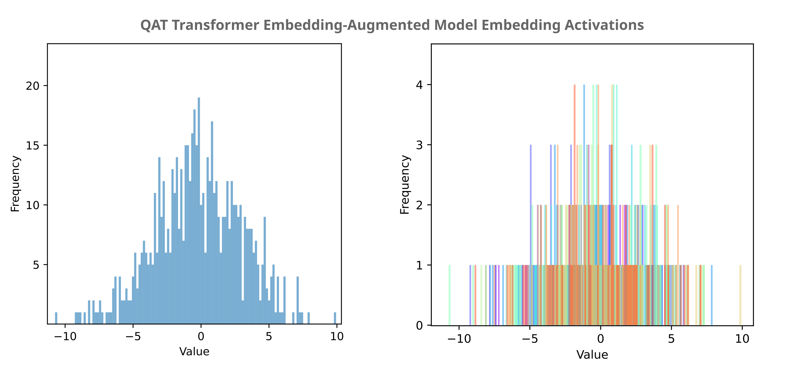
The approximately normal distribution present in these activations would be expected to account for the gap between BNB Int8() and FLoat8 E4M3fn accuracy.

When we compare the distribution of this quantization-aware model to the non-quantized-aware model, we see that the mean is still centered around the origin but the variance is larger, and the distribution is notably flattened. This is to be expected, as activation values must be pushed farther apart in order to remain distinct upon addition of the uniform noise.

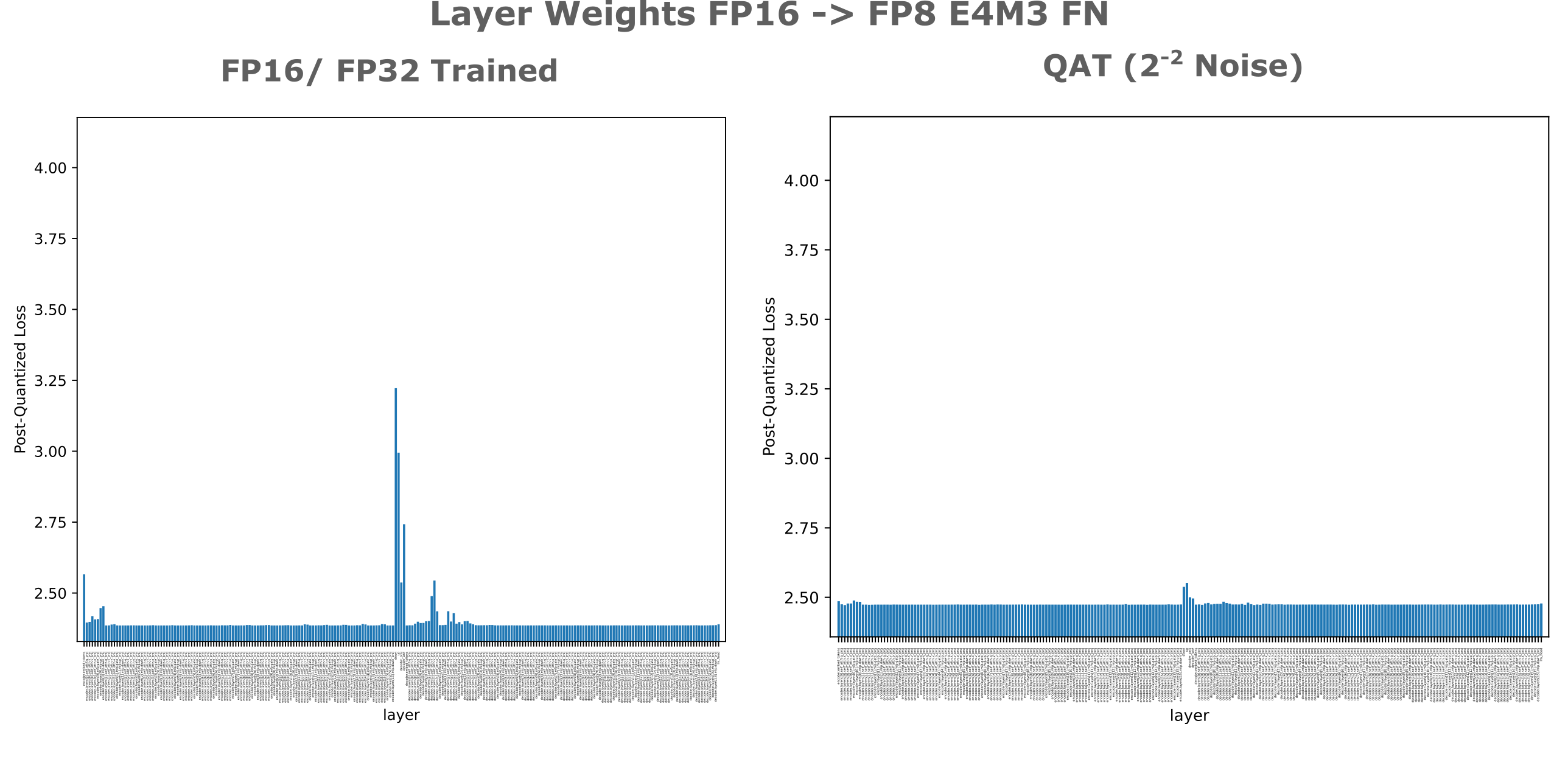
When we observe the sensitivity of each layer in a noise-induced quantization-aware trained model compared to our original full-precision model, we find something interesting: not only are activations of the layer to which we added the noise (down) no longer sensitive to 8-bit quantization, but also neither are the other layers that were found to be relatively quantization-sensitive (early transformer layers in the decoder and encoder, up projection, etc.). This suggests that injection of noise into an arbitrary model layer’s activations is capable of imparting quantization insensitivity on all layers.

This is also true of the weight layers: noise injection into the compressed embedding layer activations imports quantization insensitivity to both encoder and decoder weight layers as well as the compression layer weights.

We can hypothesize that the converse of the last statement may also be true: if noise is injected into another layer, it may result in quantization insensitivity in our vector of interest (the compressed layer activations). Rather than injecting noise directly into our compressed embedding layer, we inject before the compression (down) transformation and add a residual across the injection point. As shown in the following figure, we do indeed see quantization insensitivity in our layer of interest as well as all others in this model.

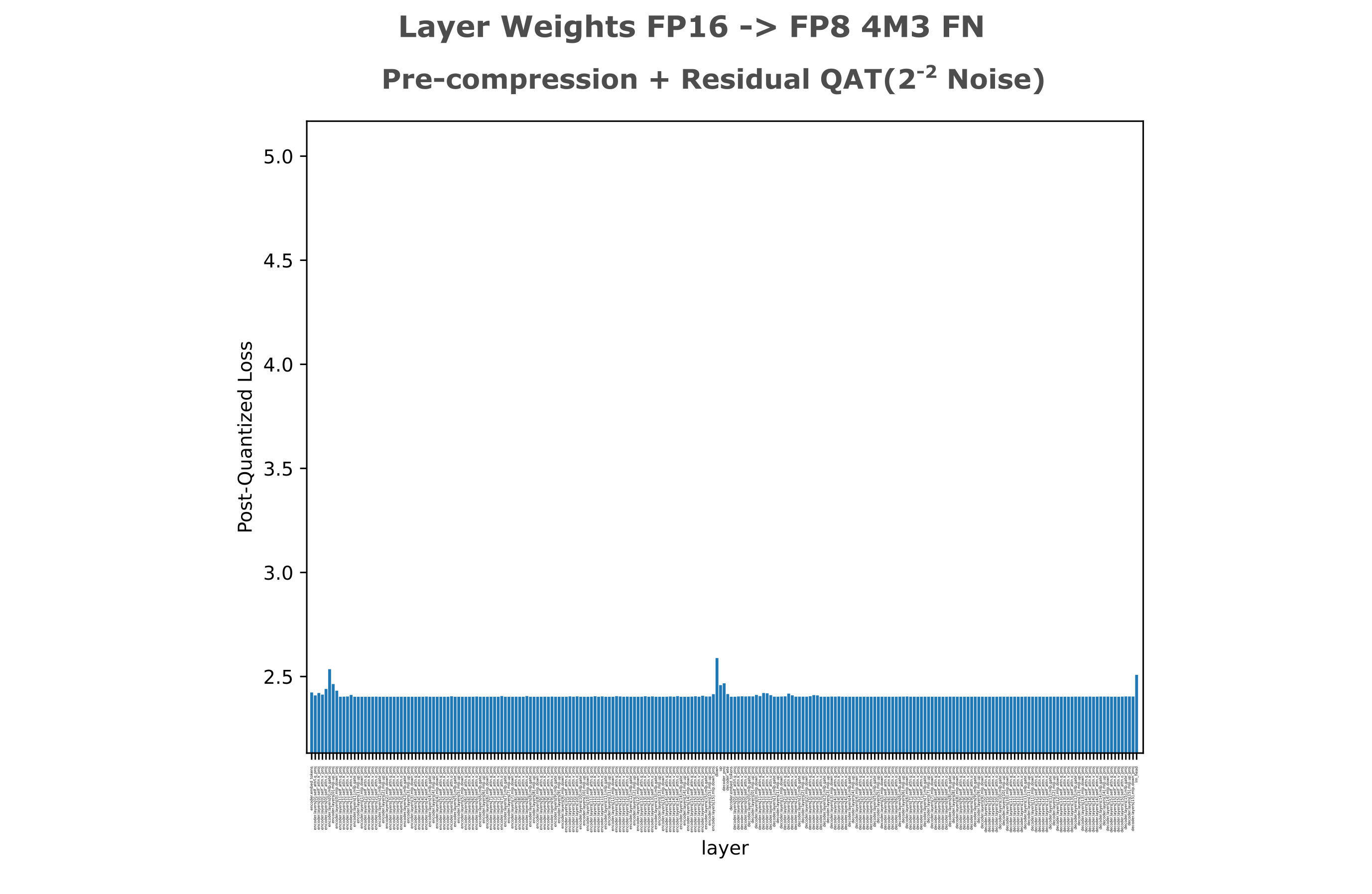
The real benefit of this approach is that it empirically results in greater quantization insensitivity in the compressed embedding, while also leading to slightly lower loss after training: the following figure shows that Bitsandbytes Int8 quantization now results in less than a 0.1% loss increase from the Float16 reference.

Embedding Datatype	Loss
Float16 (E5M10)	2.4203
BNB Int8()	2.4228
Float8 (E4M3fn)	2.4687
Float8 (E5M2)	2.6070

When we re-train noise-injected (at the compressed embedding unless otherwise noted) models and compare to a re-trained full-precision model, we find that there is a non-obvious relationship between increased noise magnitude and training efficiency. Most notably, there is little to no difference between training efficencies of the QAT model with $2^{-4}$ uniform noise injected at the compressed embedding, a model with $2^{-2}$ noise injected inside a residual before compression, or the full-precision model.

To conclude, we find that embeddings can indeed be quantized to 8 bits per parameter with no real loss difference (using BitsandBytes Int8()) from the unquantized embedding using noise-injected QAT models. As this QAT method imparts minimal increase in evaluation loss compared to full-precision training, we conclude that the compressed embeddings of a QAT model are quantizable without loss, with little to no training efficiency difference from the full-precision model training detailed previously.

Estimation of language entropy

We seen that the introduction of an (oracle) embedding into a causal decoder allows for more efficient language compression than either a standard one-pass encoder-decoder or causal decoder-only architecture. It is particularly noteworthy that embedding-augmented models exhibit different asymptotic training characteristics relative to causal decoder models: for this section, it is important to observe that causal model loss during training is well approxiated by a log-linear relationship, where a constant decrease in loss occurs upon a fixed magnitude change in training inputs (ie number of tokens or training steps). For example, if we may see a 0.4 CEL decrease upon doubling of the number of input steps, we would expect to see another 0.4 CEL decrease upon another step doubling.

Now consider the following question: how effective can language models possibly be? We can think about this in terms of both how much incompressible information language exhibits, or in terms of the intrinsic entropy present in langauge itself. To see that language does have non-zero intrinsic entropy, for any given word on this page observe that you could replace the rest of the text with an equally grammatically valid (and factually valid etc.) unique completion.

One straightforward way to estimate this intrinsic language entropy is to train large causal decoders on more and more tokens using a cross-entropy loss metric, and observe this loss after the training has converged. But even supposing that we had an arbitrarily large model capable of training on finite hardware, this approach is not computationally feasible: as long as loss curves remain log-linear, not only does convergence never actually occur but we require an exponential amount of data and compute to achieve a linear increase in estimation accuracy.

With the observation that embedding-augmented models experience linear rather than exponential decay during training, it is clear that these models are much more suitable for intrinsic language entropy estimation. The approach is straightforward, train sufficiently large encoder-augmented embedding models with smaller and smaller embedding sizes and observe the size required for convergence to 0 CEL. The smallest embedding size required for the model to achieve zero loss (on hold-out data) is the langauge entropy estimation.

Token Entropy Estimation

When large language models are trained, the current approach is to feed a large number (on the order of trillions) of tokens to these models, and doing so requires a very large amount of compute to process many forward and backward passes on this data. The paradigm of language model prediction ability scaling with the input data size has been observed since 2016 or so, and is likely to be observed further into the future as well. But the finite amount of language data available means that input data cannot be scaled without reaching a limit. More recently it has been observed that models trained on filtered data (selected for factual accuracy, informational content etc.) perform substantially better on downstream tasks such as those present in benchmarks used to measure large language models (MMLU etc).

We approach the filtering of data at a very granular level, at the token rather than passage. Given a certain passage (which we assume can be tokenized to fit in a given context window), which tokens are ‘more important’ to be trained on and which are less? This is a somewhat subjective question as it depends on what one wants a language model to do, but from the perspective of training a model to minimize language entropy there is a single answer: as no model can surpass the entropy of a conditional next token, training should be performed such that the model’s weights are not modified in order to attempt to do so. It is clear that attempting to train a model past each token’s intrinsic entropy is impossible, and in practical terms is a waste of compute and data.

How can one perform this entropy-aware training? The first step is to be able to estimate what the entropy of each (conditional) token is, and happily model to be able to do so in an efficient manner: the embedding-augmented causal decoder model presented above. To see why this is the case, first observe that any model trained for causal language prediction yields an entropy estimation for each conditional token, which is the model’s cross-entropy loss on that token. The lower the model’s loss across all tokens (which is usually mean reduced) the more accurate this entropy estimate is, such that the embedding-augmented entropy prediction model is a more accurate token entropy predictor than a purely causal model.

What if we train a strong entropy prediction model such that the causal decoder obtains near-zero loss with a minimal embedding size, how then can we estimate each token’s conditional entropy? Or even if this case is not met, how do we compute the conditional entropy of any given token using entropy estimation models, as the entropy estimation occurs over many tokens rather than one?

It may be wondered why one cannot simply train an entropy estimation model to minimal average loss, observe the unreduced cross-entropy loss for each token with this trained model, and simply add the amortized embedding’s entropy (in bits) to this loss value. This value will unfortunately be inaccurate for most tokens, however, as we cannot a priori know how many bits in the embedding correspond to each individual token. Recall that the intrinsic entropy in a sequence $x$ is equivalent to the minimal embedding’s amortized bits divided by the number of bits in the sequence (see the following). In that case, we average over all elements of $x$ during the amortization process; for token-specific entropy estimation, we want to find out exactly how the bits in the embedding are distributed exactly among tokens.

\[H(x_0, x_1, ..., x_{i-1}) = \vert e \vert + \sum_i H(O(x_{:i-1}, \theta_d), x_i)\]

Unfortunately this decomposition at the level of the token is difficult if we restrict ourselves to one model alone: we cannot simply remove the encoding and inference the decoder to find the left over entropy being that the encoding is not linearly separable from the rest of the decoder’s inputs (as the decoder is itself a nonlinear function).

To find a given token’s conditional entropy exactly, we can instead use two models such that one entropy estimation model $\theta_1$ has a context window of size $N-1$ and the other $\theta_2$ has a context window of size $N$. With these models, we proceed in a different manner depending on whether or not we have a fixed encoder size $\vert e \vert$ (in bits) such that the model’s cross-entropy loss for each segment of text is $\Bbb L \geq 0$ or a variable-size $\vert e \vert$ such that each segment of text has $\Bbb L = 0$. The latter would require a very subtle implementation in a single model, or many training runs using many fixed-size models, so we focus on the former as a more realistic scenario.

Thus we have the following: two entropy estimation models, $\theta_1$ with context window $N-1$ and $\theta_2$ with context window $N$, and for simplicity we assume that the embeddings of these models are the same size, $\vert e_1 \vert = \vert e_2 \vert$ although this is certainly not a necessary condition. We can then compute the entropy of the token at position $N$ given the tokens at position $0, 1, …, N-1$ using these models as follows (denoting the sequence of tokens $(t_0, t_1, …, t_N)$ as t_{:N}$)

\[H(t_{N} \vert t_{:N-1}) = H(t_{:N}) - H(t_{:N-1}) \\ = H \left( O((t_{:N-1}, \theta_2), (t_{:N}) \right) - H \left( O((t_{:N-2}, \theta_2), (t_{:N-1}) \right) \\ = \vert e \vert + \sum_{i=0}^N \Bbb L(O(t_{:i-1}, \theta_2), t_i) - \left( \vert e \vert + \sum_{i=0}^{N-1}\Bbb L(O(t_{:i-1}, \theta_1), t_i) \right) \\ = \sum_{i=0}^N \Bbb L(O(t_{:i-1}, \theta_2), t_i) - \sum_{i=0}^{N-1}\Bbb L(O(t_{:i-1}, \theta_1), t_i)\]

which if we use reduced cross-entropy losses for both models,

\[H(t_{N} \vert t_{:N-1}) = \sum_i^{N} \Bbb L (O(t_{:i}, \theta_2) - \sum_{i=0}^{N-1}\Bbb L \left( O(t_{:i}, \theta_1) \right)\]

This follows from the chain rule of conditional entropy,

\[H(C \vert A, B) = H(A, B, C) - H(A, B)\]

To use this method in practice, we would slide two windows across the text corpora as follows:

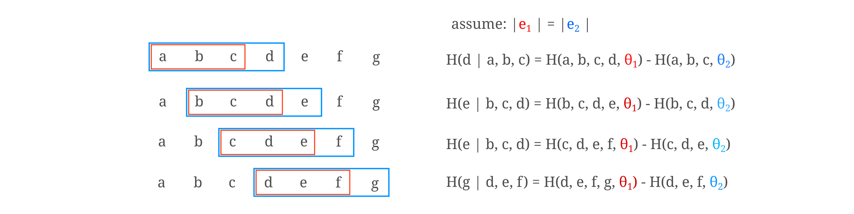
Instead of using two models, one can instead use one model and simply mask the first token and shift the $\theta_2$ model’s context to start at the $t_{-1}$ index and proceed with the calcluation above. We assume that the model is trained using left padding and that not all inputs are of length $n_{ctx}$ before padding such that the encoder and encoder have been exposed to pad tokens during the training process. In this single-model formulation, the calculation of the conditional entropy of token $t_N$ is as follows:

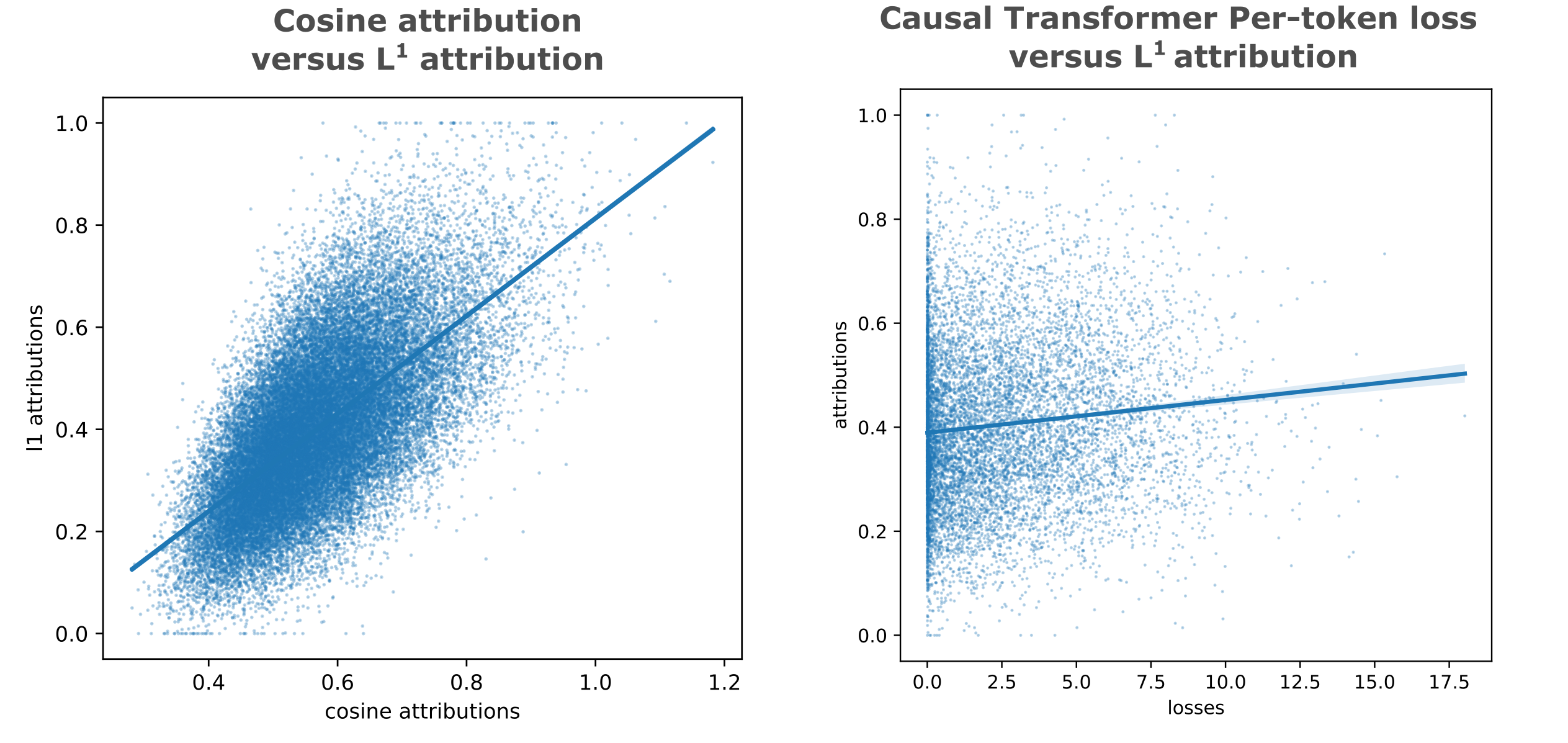
\[H(t_{N} \vert t_{:N-1}) = \Bbb L (O(t_{0:N-1}, \theta), t_{1:N}) - \Bbb L \left( O(t_{-1:N-2}, \theta), t_{0, N-1} \right)\]

We also investigate ways to efficiently estimate the token entropy given an embedding-augmented causal model: we can observe how much each output depends on the encoder’s embedding, reasoning that lower entropy tokens will be less sensitive to encoder information loss. What we want is essentially a measure of input attribution, to be specific the attribution of all outputs to the embedding input. One way to calculate this attribution is by simply masking the embedding and measuring the change in output upon doing so, which is known as occlusion. This approach has a particularly beneficial property for our purposes: as we want to measure the effect of one input on all outputs, we can compute the occlusion value with only two forward passes (without forming gradients) per text segment. We can calculate the occlusion value using our entropy estimation model as follows:

\[x = O(x, \theta_e) \oplus W_{wte}x \\ x_o = \mathbf{0} \oplus W_{wte}x \\ Attr(x) = m(O(x, \theta_d), O(x_o, \theta_d))\]

where $W_{wte}$ is the decoder’s word token embedding transformation, not the encoder’s, and $\oplus$ signifies concatenation (in this case in the sequence dimension), $\mathbf{0}$ the zero vector, $\theta_e$ the encoder model, and $\theta_d$ the decoder. In addition to occluding the memory input, we apply an attention mask to that input as well for transformer models.

THere are a number of options we can use for our metric: a Banach space norm like $L^1$ or $L^2$, cosine similarity, a max norm, or even quantity that is not strictly a matric on a space at all such as

\[m_{l^1}(O(x, \theta_d), O(x_o, \theta_d)) = || O(x, \theta_d) - O(x_o, \theta_d) ||_1 = \sum_i | O_i(x, \theta_d) - O_i(x_o, \theta_d) |\]

where $i$ is indexed in the embedding dimension. Here we actually use the logit activations rather than the embeddings, so effectively $m_{l^1}$ measures the Manhattan metric bewteen the decoder’s logits with versus without the encoder’s embedding. For transformers, we can remove the embedding using an attention mask.

An $L^1$ norm is sensitive to changes in scale between samples, which can be a problem as gradient descent is normally calculated batchwise such that scale inequalities between samples in a batch lead to biases in gradient magnitude once weights are applied. To normalize all token attributions to take values in $[0, 1]$, we use a simple linear minmax approach,

\[N_{minmax}(y) = \frac{y_j - \mathrm{min} \; y}{\mathrm{max}\; y - \mathrm{min} \; y }\]

where $j$ iterates on the sequence dimension, and $\mathrm{max}, \mathrm{min}$ are computed on this dimension as well. We mask all pad input elements during this normalization process, such that these are assigned infinite values for minimum computation and zero values for maximum computation (the norms of the actual $y$ values are usually >10000, and none have zero distance due to their very high dimensionality).

We can also use the complement of the cosine similarity (distance) as our metric, and to remain consistent with our $L^1$ metric introduced earlier we use the complement of the cosine distance,

\[m_{cosine}(O(x, \theta_d), O(x_o, \theta_d)) = 1 - \frac{O(x, \theta_d) \cdot O(x_o, \theta_d)}{|| O(x, \theta_d) || \; || O(x_o, \theta_d) ||}\]

This metric has the advantage of not needing to be normalized, as the range is $m_{cosine}(O(x, \theta_d), O(x_o, \theta_d)) \in [0, 2]$ with nearly all values in $[0, 1]$ for sufficiently high-dimensinoal output vectors.

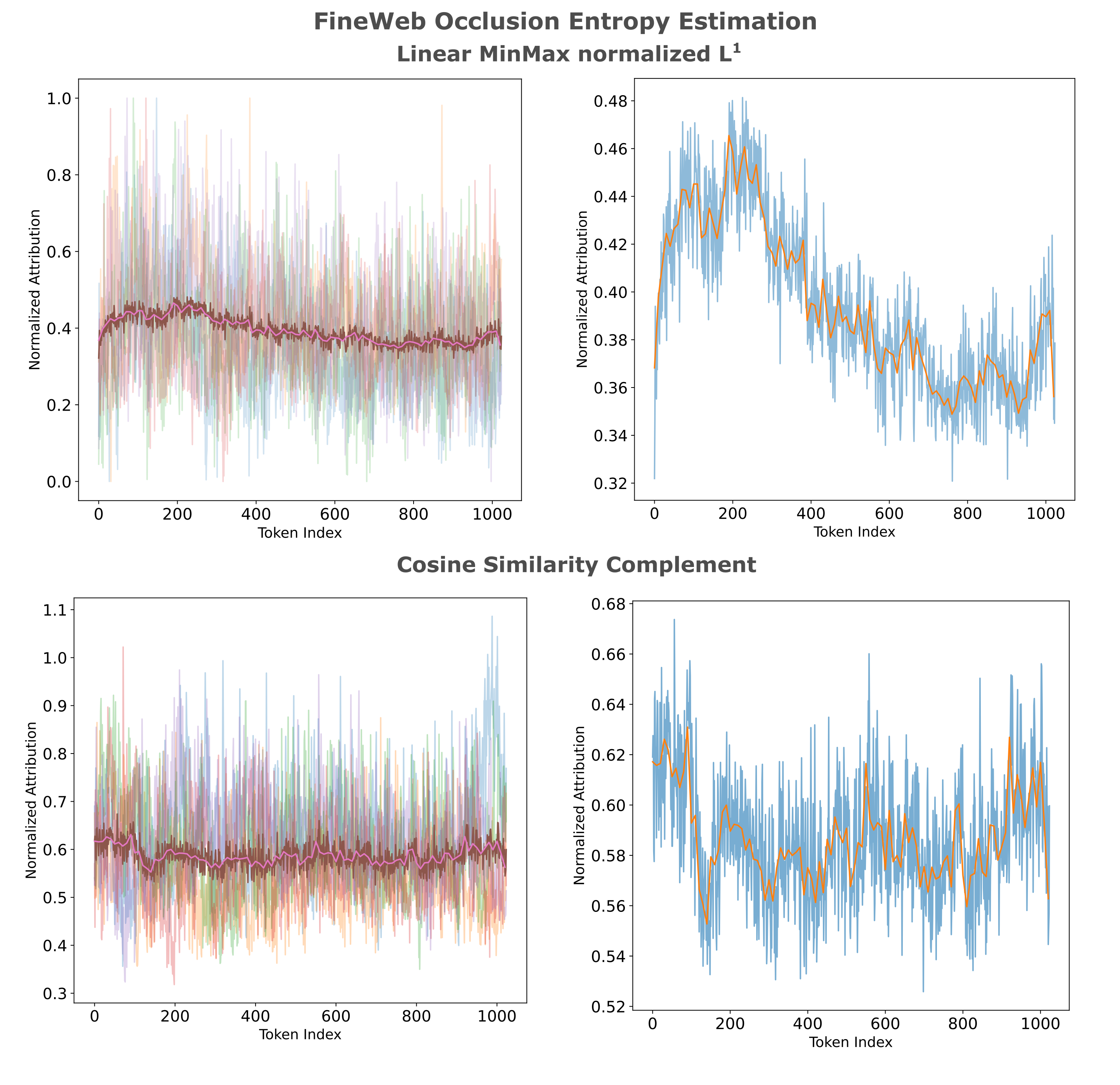
Which metric is more effective in extracting the model’s estimate of the source entropy? We can observe the attributions placed on each token of a given corpus for both attributions to investigate this question. Visualization can be accomplished by highlighting (in red) the decoded characters of tokens that receive more embedding attribution, ie have a higher source entropy estimation. As attributions are calculated for outputs of a given token (which correspond to the next token prediction for causal models), we right-shift the attributions one index so that the color a token is highlighted corresponds to the attribution of the model’s prediction of that token. For the $L^1$ attributions, we have the following (truncated from the 1024 tokens of the full text for brevity:

CTComms sends on average 2 million emails monthly on behalf of over 125 different charities and not for profits. Take the complexity of technology and stir in the complexity of the legal system and what do you get? Software licenses! If you've ever attempted to read one you know how true this is, but you have to know a little about software licensing even if you can't parse all of the fine print. By: Chris Peters March 10, 2009 A software license is an agreement between you and the owner of a program which lets you perform certain activities which would otherwise constitute an infringement under copyright law. The software license usually answers questions such as: The price of the software and the licensing fees, if any, are sometimes discussed in the licensing agreement, but usually it's described elsewhere. If you read the definitions below and you're still scratching your head, check out Categories of Free and Non-Free Software which includes a helpful diagram. Free vs Proprietary: When you hear the phrase "free software" or "free software license," "free" is referring to your rights and permissions ("free as in freedom" or "free as in free speech").

And for the same corpus using the cosine similarity complement metric, we have

CTComms sends on average 2 million emails monthly on behalf of over 125 different charities and not for profits. Take the complexity of technology and stir in the complexity of the legal system and what do you get? Software licenses! If you've ever attempted to read one you know how true this is, but you have to know a little about software licensing even if you can't parse all of the fine print. By: Chris Peters March 10, 2009 A software license is an agreement between you and the owner of a program which lets you perform certain activities which would otherwise constitute an infringement under copyright law. The software license usually answers questions such as: The price of the software and the licensing fees, if any, are sometimes discussed in the licensing agreement, but usually it's described elsewhere. If you read the definitions below and you're still scratching your head, check out Categories of Free and Non-Free Software which includes a helpful diagram. Free vs Proprietary: When you hear the phrase "free software" or "free software license," "free" is referring to your rights and permissions ("free as in freedom" or "free as in free speech").

It is worthwhile to check and see how reasonable these entropy estimations are, and one way we can do this is to observe the words that tend to have higher or lower entropy estimation in the above corpus. This sort of analysis is of limited benefit to the actual modeling process, as deep learning as a discipline may be thought of as foregoing such rule-based models for models that learn their own rules from arbitrary starting points, but is useful for checking to see if our model we are using here is at all capable of the kind of entropy estimation we want.

The first observation is that for words that are split into more than one token, the attribution of the first token is usually large than the second. This is what we expect, as there is often far fewer degrees of freedom for a word once a few letters have been provided. Secondly, words that are more or less unpredictable (the author of this passage, the title of an external work etc.) receive a higher attribution than those that are perhaps more predictable such as those that relate to the subject of the passage itself.

It is clear that the attributions as measured by an $L^1$ metric are substantially similar to those obtained using the cosine similarity complement, although there is a larger dynamic range for $L^1$ data. It seems justified therefore to simply choose one (or a combination of both) and proceed.

It is interesting to take some time to observe some general statistics on the relationship between token index and entropy. We can guess that tokens existing early in a corpus will in general have higher attribution to the embedding (ie higher entropy) than later tokens as there are more degrees of freedom early in a given corpus. We find that his is indeed the case when we look at attribution values from 80 random samples,

Besides occlusion, there is another way to measure attribution: we can forward propegate from the input $x$, back-propegate all the way back to $x$, and multiply the gradient of $x$ by the value of $x$. This effectively measures the sensitivity of the model to a very small change in the input, as opposed to a large change that we observe with occlusion. This is somewhat unimaginatively commonly termed ‘gradientxinput’.

The use of this method for our entropy estimation requires a few extra steps, partially because we want to find the attribution of all outputs with one input (rather than one output with all inputs as is normally the case) and partially because we don’t want to actually backpropegate to the input rather only the encoder’s output (which is an embedding of floats). We can backpropegate the $L^1$ norm of the output as follows:

\[Attr(x_i) = \nabla_{O(x, \theta_e)} \sum_j | O(O(x, \theta_e) \oplus x_{:i-1}, \theta_d))_{j, i} | \circ O(x, \theta_e)\]

where $A \circ B$ signifies the Hadamard product of A and B, and $x_{:i-1}$ the tokens of $x$ indexed by $i$ and the embedding dimension is indexed by $j$. Note that we cannot reduce the gradients formed on the output tokens $0, 1, 2, …, i$ before backpropegating, as we need to keep the token gradients separate in order to determine attribution of each with respect to the embedding (we do reduce across the batch dimension as these elements are separable). This results in a very large time complexity penalty when using this method compared to occlusion: we need to perform $N$ backwards passes for $N$ tokens of one sequence, making this method around a thousand times less efficient than occlusion. As before, we perform minmax normalization on the raw outputs of $Attr(x_i)$.

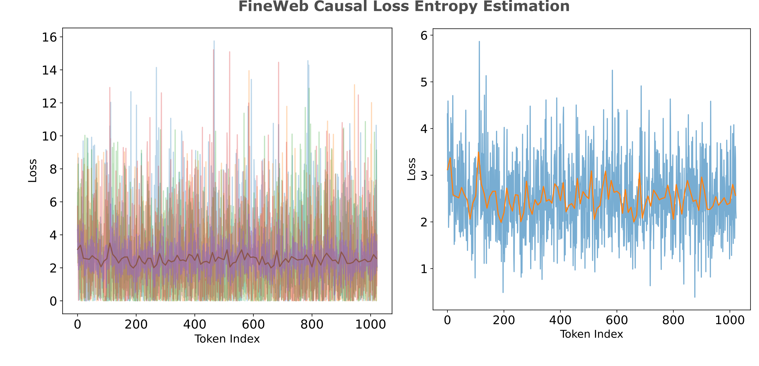
CTComms sends on average 2 million emails monthly on behalf of over 125 different charities and not for profits. Take the complexity of technology and stir in the complexity of the legal system and what do you get? Software licenses! If you've ever attempted to read one you know how true this is, but you have to know a little about software licensing even if you can't parse all of the fine print. By: Chris Peters March 10, 2009 A software license is an agreement between you and the owner of a program which lets you perform certain activities which would otherwise constitute an infringement under copyright law. The software license usually answers questions such as: The price of the software and the licensing fees, if any, are sometimes discussed in the licensing agreement, but usually it's described elsewhere. If you read the definitions below and you're still scratching your head, check out Categories of Free and Non-Free Software which includes a helpful diagram. Free vs Proprietary: When you hear the phrase "free software" or "free software license," "free" is referring to your rights and permissions ("free as in freedom" or "free as in free speech").

It is also worth observing how the attribution values obtained above relate to the (normalized) loss per token we get when we inference a purely causal model trained on the same data. For a perfect causal model, the cross-entropy loss values per token are the text’s intrinsic entropy values and are the same as the information a decoder requires per token from an oracle embedding for our entropy estimators. We have far from perfect models, however: the causal transformer used to estimate token losses below achieves an average CEL of 2.5, meaning that the model achieves a bits per byte compression of

\[\mathtt{bpb} = \frac{L_t / L_b * \Bbb L}{\ln 2} \approx 0.920\]

which is far less than state-of-the-art models like Deepseek V3, which achieve <0.5 BPB on similar datasets. This means that the majority of this model’s loss is not due to intrinsic entropy of language but instead to the difference between the model’s probability distributions and the underlying data. Nevertheless, we can perform entropy estimation using this model, and highlight the same text segment (again using red for higher and green for lower entropy).

CTComms sends on average 2 million emails monthly on behalf of over 125 different charities and not for profits. Take the complexity of technology and stir in the complexity of the legal system and what do you get? Software licenses! If you've ever attempted to read one you know how true this is, but you have to know a little about software licensing even if you can't parse all of the fine print. By: Chris Peters March 10, 2009 A software license is an agreement between you and the owner of a program which lets you perform certain activities which would otherwise constitute an infringement under copyright law. The software license usually answers questions such as: The price of the software and the licensing fees, if any, are sometimes discussed in the licensing agreement, but usually it's described elsewhere. If you read the definitions below and you're still scratching your head, check out Categories of Free and Non-Free Software which includes a helpful diagram. Free vs Proprietary: When you hear the phrase "free software" or "free software license," "free" is referring to your rights and permissions ("free as in freedom" or "free as in free speech").

Here we see some of the same qualitative features as we saw using $L^1$ and cosine attribution: for words composed of two or more tokens, the first token is invariably of higher entropy, less entropy for articles, etc. On the other hand, there is less shift in average entropy per index across our context window.

When we observe statistics across many samples, we find that there is a strong correlation between $L^1$ and cosine similarity attribution ($R^2=0.42$), but little correlation between $L^1$ attribution and (normalized) loss per token ($R^2=0.01$).

There is somewhat stronger correlation when we compare the occlusion attribution of an embedding-augmented model that achieves low loss (CEL < 0.4) using a large $d_m=1024$ embedding (Large Embedding in the table below), but attributions for this embedding or embeddings from even larger models (same $d_m$, double the layers in both encoder and ecoder for CEL < 0.1) do not correlate strongly with the small-embedding model.

y vs x	$m$	$b$	$R^2$
$L^1$, cosine	0.9566	0.1431	0.4195
$L^1$, loss	0.0063	0.3894	0.0107
Large embedding $L^1$, loss	0.0172	0.4152	0.0688
Large embedding $L^1$, $L^1$	0.2308	0.3691	0.0424
Largest embedding $L^1$, $L^1$	0.2680	0.3629	0.0574

We find much stronger correlation between exact entropy estimations via single model pad-based decomposition and the small causal model’s losses ($R^2 = 0.3285$, below left). While it remains possible that a very strong entropy estimation model would yield similar entropy values for embedding occlusion-based entropy to a similarly strong causal language model, these results suggest that for our compute attribution-based esimates are not accurate.

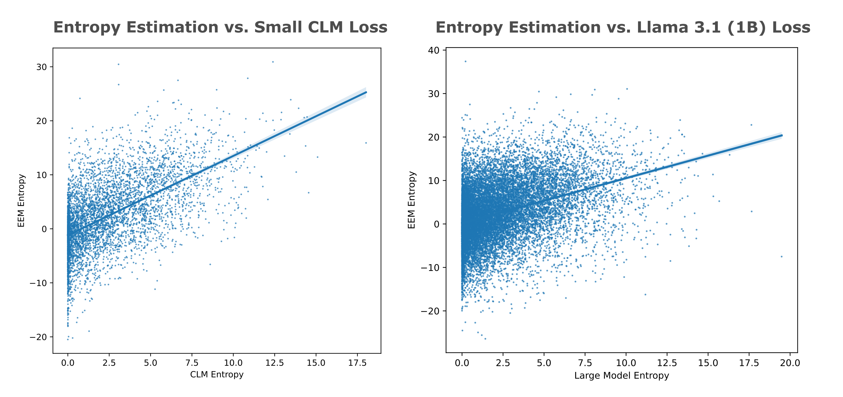
How can we simulate the use of a strong entropy estimation model without dealing with the compute required to train this model or inference for entropy token estimations? One option is to use a causal model that has had an enormous amount of compute (around 100,000x what the models here have seen) applied during training in place of an entropy estimation model. This large compute results in significant differences in entropy estimation accuracy (or equivalently compression): for example, the small causal model above achieves 1.29 BPB on Wikitext, but the larger and heavily trained Llama 3.2 (1b) reaches 0.66 BPB on the same dataset.

The main difficulty with this approach is that these models use a different tokenizer: the Llama 3.2 model uses a 128k size tokenizer compared to the 8k size tokenizer used by the small models. To find the entropy estimations (losses) for the smaller tokenizer, we proceed as follows: first the losses per token are found for the large tokenizer, then the losses are applied to each character, and finally the average loss per character is found when characters are grouped according to the small tokenizer.

This conversion is necessarily somewhat lossy: we cannot be sure that the entropies for sub-token elements (characters in this case) would all be equal to the entropy of the token as a whole, and in many cases it is convincing that most elements would not be equal to the token entropy. Nevertheless, this method provides some notable advantages over the alternative of retraining a large model to use a different tokenizer, namely that model performance tends to plummet when tokenizers are retrained from scratch.

When we perform this tokenization conversion to render the causal losses (entropy estimates) of Llama 3.2 (1B) in the 8k tokenizer we have been using elsewhere on this page, we find the following for our favorite text segment:

CTComms sends on average 2 million emails monthly on behalf of over 125 different charities and not for profits. Take the complexity of technology and stir in the complexity of the legal system and what do you get? Software licenses! If you've ever attempted to read one you know how true this is, but you have to know a little about software licensing even if you can't parse all of the fine print. By: Chris Peters March 10, 2009 A software license is an agreement between you and the owner of a program which lets you perform certain activities which would otherwise constitute an infringement under copyright law. The software license usually answers questions such as: The price of the software and the licensing fees, if any, are sometimes discussed in the licensing agreement, but usually it's described elsewhere. If you read the definitions below and you're still scratching your head, check out Categories of Free and Non-Free Software which includes a helpful diagram. Free vs Proprietary: When you hear the phrase "free software" or "free software license," "free" is referring to your rights and permissions ("free as in freedom" or "free as in free speech").

There are broad similarities to the small model losses on this page, and when we plot average loss per token index we find the strongest match to our prior expectation of high loss at the start of a sequence:

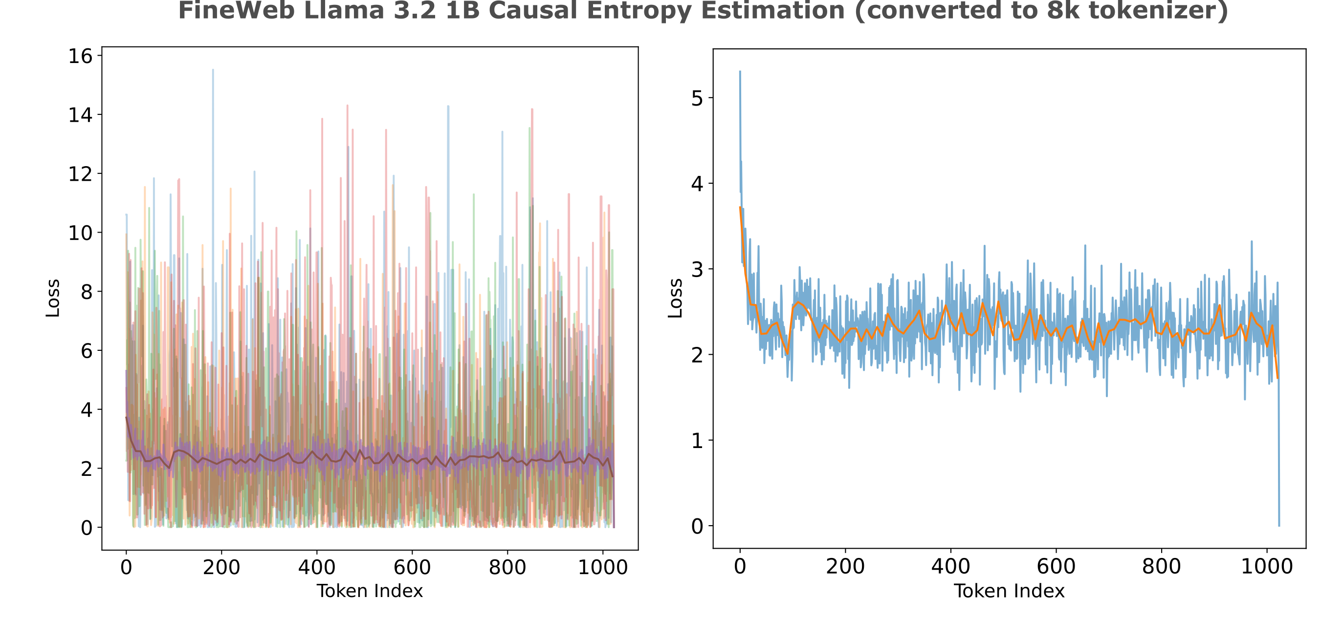
We find a relatively strong correlation ($R^2 = 0.4922$) between token losses obtained from our smaller model and the converted losses from the large one, and a somewhat weaker correlation between the entropy estimation model’s estimations and large model losses ($R^2 = 0.1360$).

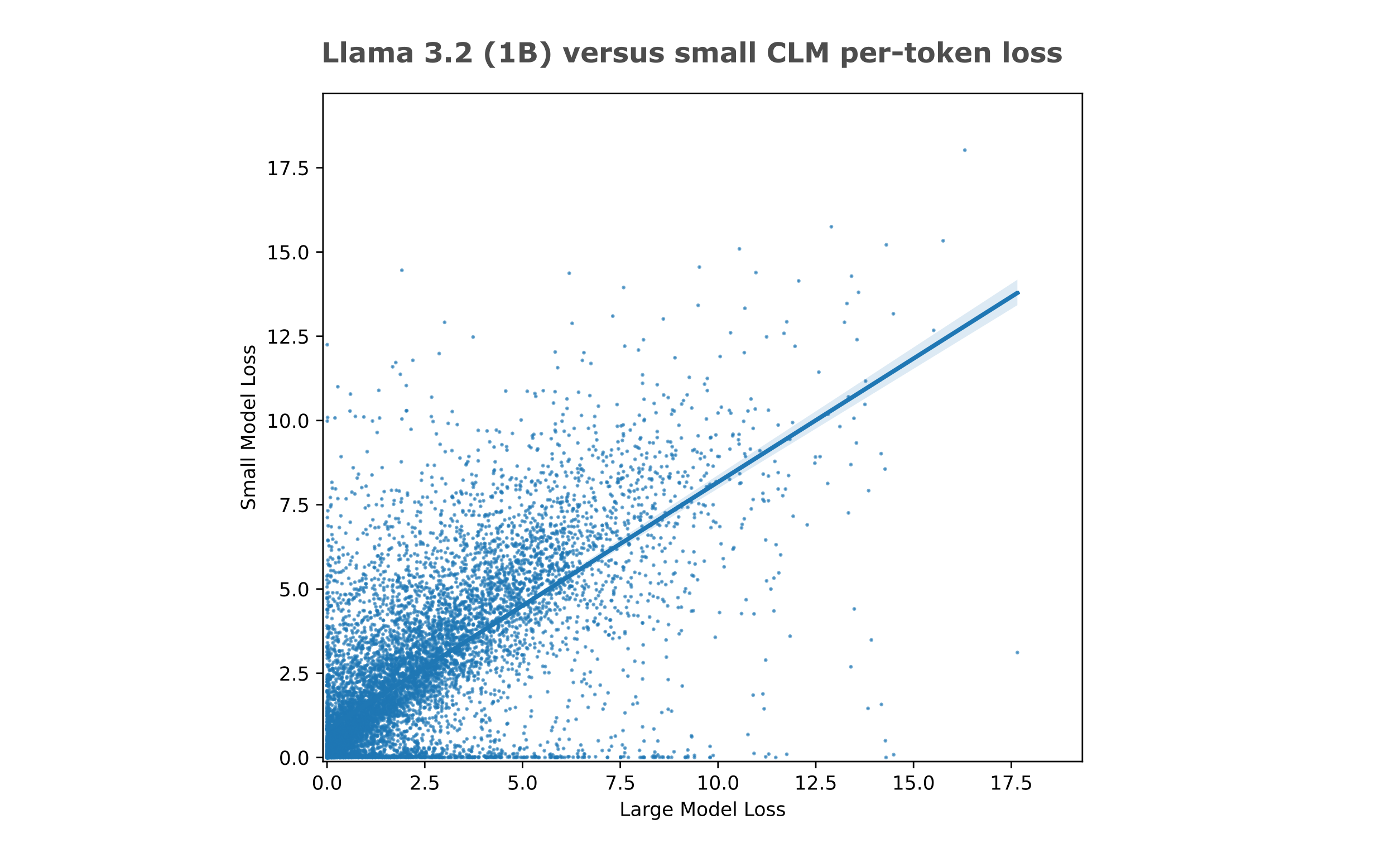
y vs x	$m$	$b$	$R^2$
Entropy Estimation, Small CLM	1.4685	-1.1879	0.3285
Entropy Estimation, Large CLM	1.0540	0.1097	0.1424
Small CLM, Large CLM	0.7334	0.8398	0.4922

All this to say that both $L^1$ or cosine metric-based occlusion attribution as well as causal per-token loss exhibit some expected statistical properties of an entropy estimator, but while an $L^1$ metric may be substituted for a cosine similarity metric for attribution, there is little to no correlation between attribution-based and loss-based entropy estimations.

Once the relative token entropy is estimated, the next step is to incorporate this information into the training algorithm such that the model is only marginally modified to fit the high-entropy tokens, while low-entropy tokens are more strongly fit. For normalized estimations, one way to do this is to assign weights to be the complement of our relative entropy values ($w_i = 1 - e_i$) such that larger loss weights are assigned to tokens with lower entropy. The idea here being that at the start of training, models predict all tokens with high entropy (see the cross-entropy loss at the start of training). Tokens that have high conditional entropy require less modification of this initial model state than tokens of low entropy, and thus smaller steps in the model’s weights for these tokens relative to low-entropy tokens result in the model reaching the intrinsic entropy loss value for both tokens, assuming that model weight modification scaling is proportional to the scaling of loss per token.

Weighting tokens by entropy estimates is notably a different concept from a standard cross-entropy loss weight, as there weights are applied per category (token for language modeling) whereas in this case we want to weight by token sequence index rather than token identity. One way we obtain a total loss from the linear combination of these weighted unreduced losses as follows:

\[\Bbb L (O(x, \theta), y) = \sum_i w_i*\Bbb L(O(x_{:i-1}, \theta), y_i)\]

Alternatively, we can rescale the loss itself, for example

\[\Bbb L (O(x, \theta), y) = \sum_i || \Bbb L(O(x_{:i-1}, \theta), y_i) - e_i ||_1\]

Taking a step back, does it make sense to modulate a model’s loss in a per-token manner when training? What we are effectively attempting is to perform a kind of model distillation, in which a strong model is used to increase some metric of goodness in a weaker one. This is commonly done today by generating text using a large model and then training a small model on that text, for example to increase chain-of-thought reasoning abilities in that small model. Our strong model here is the entropy estimation model, and as this model is not strictly generative we cannot use an analagous method. We get two outputs from the entropy estimation models: tokens predicted, and entropy per token. As we cannot use the token prediction for generation, we must use the entropy per token. But what can this token entropy do to help a causal model’s training?

One approach to language modeling is to simply train on everything you can get your hands on, with the idea that a model can ‘soak up’ the data and will perform better than when trained on curated data. This is an inefficient way to train models, however, as it has been shown numerous times in recent years that models trained on filtered data (in this case signifying selection of text documents from a broad corpus, for example choosing educational documents from a Common Crawl snapshot) far outperform models trained on unfiltered data (in the previous example, all data from the common crawl). The reason for this is that it is not inaccurate to think of a model as a sponge that can indeed ‘soak up’ the training data, but that this sponge is finite in size and can only soak up so much given a fixed amount of compute or data. In this analogy, we want the model to attempt to learn the aspects of a dataset that indeed learnable, rather than the ones that are fundamentally un-learnable. In this sense we want to spend compute on learning to predict the predictable tokens, not the stochastic ones that have high entropy.

In many ways the idea that one should only update a model with non-stochastic information is not new, and in one way or another has worked its way into many aspects of modern models. One notable example is the widespread use of the Adam and AdamW optimizers: the original goal of these adaptive optimizers was to deal with noisy data, and indeed they tend to outperform other adaptive optimizers when models are trained on data with a certain threshold of noise. The main idea here is that these most of those methods use heuristics (for example, optimizers tend to filter noise by using second moments) whereas if we know the ‘true’ entropy of each token then we have an information-theoretic optimal basis for optimization.

Our first hypothesis therefore is that training a causal model on entropy-informed data will be more efficient relative to loss per compute applied compared to training a model on the same dataset without the entropy data. To test this, we can train a small model on data with and without entropy information and observe the resulting loss curves.

Secondly, we can almost by definition expect for a causal model trained with rescaled loss to be more or less totally resistent to overfitting. This is in itself a useful application of entropy models as the usual method of preventing overfitting (evaluating on a hold-out data sample and taking a training checkpoint with the lowest evaluation loss) leads a number of difficulties: firstly one cannot train on the hold-out dataset, secondly one must assume that the hold-out data is identically and indepentently distributed to the training data (which is not always the case), and thirdly hold-outs become unreliable when they are used to optimize architectures or data sources as they effectively become the metrics one optimizes for and are thus themselves prone to overfitting.

Entropy-informed models generalize better

But this is not the only utility provided by using rescaled losses with respect to overfitting: not only can we do away with hold-out datasets, but we can also expect for a model trained using entropy information to be more generalizable than a model trained without entropy information. To see why this is the case, consider the extreme case of a model trained on a single short token sequence. Without entropy information, we can expect for predictions for each token to be more or less equally optimized at each step (assuming a random initialization of our model) whereas with entropy information each token prediction is optimized according to the entropies provided. This means that these two models will embark on very different trajectories during training, where the generalization of the entropy-less model will be expected to be lower than the entropy-informed model even before the entropy estimation losses are achieved.

Does it matter if a model is trained past the entropy of its training dataset? We can prove that such models will necessary exhibit higher hold-out test dataset cross-entropy loss (ie lower generalization) than models that are not trained to do so.

Theorem: Generalization decreases when models are trained to minimize their losses below the entropy of the training dataset.

Proof: We assume that some random variable $X$ exists and is sampled independent and identically distributed disjoint subsets, $X_{train}$ and $X_{text}$, where ${X_{train}} \; \bigcup \; {X_{test}} = {X}$ and ${X_{train}} \; \bigcap \; {X_{test}} = \emptyset$. For notational simplicity, we substitute $s = X_{train}$ and $t = X_{test}$. We assume that the entropy of the random variable is nonzero, $H(x) > 0$, and by the independence of $s, t$ we have $H(x) = H(s, t) = H(s) + H(t)$. We also assume that model losses for random variables $s, t$ are cross-entropies on causal predictions, ie $1/i\sum_i\Bbb L(O(s_{[:i-1]}, \theta), s_i) = H(O(s, \theta), s)$ and the same for $t$.

From Gibbs’ inequality, we know that $H(O(x, \theta), x) \geq H(x) \; \forall x, \theta$. We decompose $x$ according to the independence of its subsets $s, t$ as follows:

\[H(O(s, \theta), s) + H(O(t, \theta), t) \geq H(s, t) = H(s) + H(t) \implies \\ H(O(s, \theta), s) - H(s) + \left( H(O(t, \theta), t) - H(t) \right) \geq 0\]

Therefore as $\theta$ is modified such that $H(O(s, \theta), s) - H(s) < 0$ decreases, $H(O(t, \theta), t) - H(t)$ increases so that the inequality above holds. We assumed that $H(t)$ is fixed, so necessarily $H(O(t, \theta), t)$ increases as $H(O(s, \theta), s)$ decreases past $H(s)$.

In fact, due to the identical distribution of $s, t$ we know that $H(s) = H(t)$ and can put a lower bound on the loss of generalization,

\[H(O(s, \theta), s) - H(s) \geq - \left( H(O(t, \theta), t) - H(s) \right)\]

We conclude by restating the above equation in words: as the left side of the inequality is negative when $H(O(s, \theta), s) < H(s)$ which was previously assumed, the difference between the model’s cross-entropy loss and the training dataset’s entropy is at least as large as the difference between the test loss and the training entropy. $\square$.

Benchmark performance with and without entropy

It may also be conjectured that training a causal model on entropy-informed data would have different qualitative characteristics as well. The idea being as follows: for a given loss per token sequence the model may achieve varying losses or more importantly here accuracies per token.

This idea is supported experimentally: if we train a $d_m=512, n_l=16$ llama-style transformer model on FineWeb-10BT and then repeat the training with the same model architecture but now using our entropy-weighted dataset, we have the following:

Model	Wikitext BPB (↓)	SWAG	HellaSwag	Arc Easy	MathQA	GLUE	Lambada OpenAI	GSM8k	Winograd	Truthful QA	Ifeval
Reference	1.2887	0.3712	0.2963	0.4933	0.2231	0.5015	0.2490	0.0159	0.5381	0.3963	0.1183
$L^1$ Attr	1.3025	0.3731	0.2994	0.4979	0.2228	0.5133	0.2546	0.0190	0.5572	0.4155	0.1238

It is interesting to note that the model trained on $L^1$ attribution-weighted data actually yields lower Wikitext compression than the reference model: this likely results from the lack of correlation between $L^1$ attribution and per-token loss.