Sine-Cosine grid map

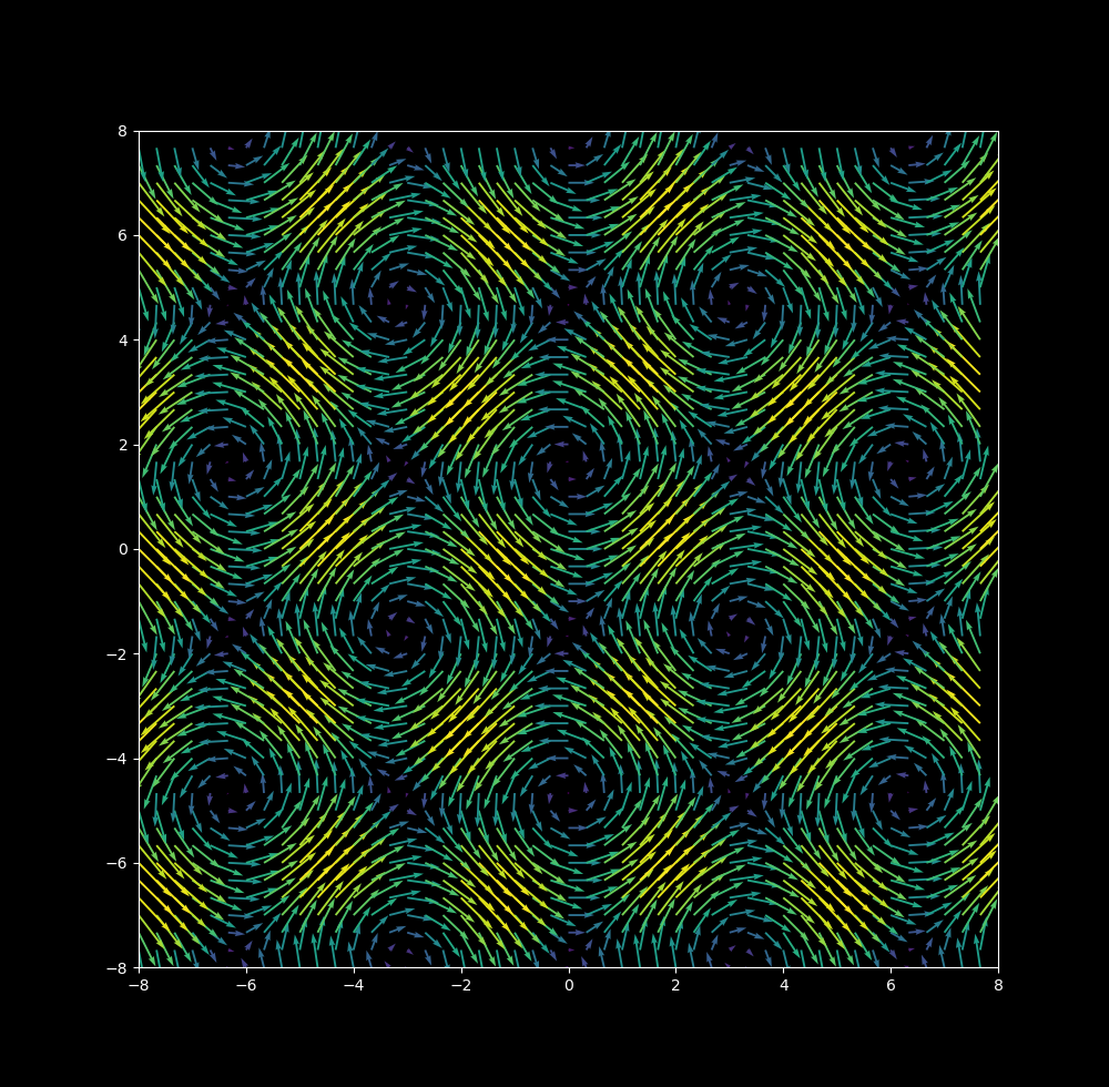
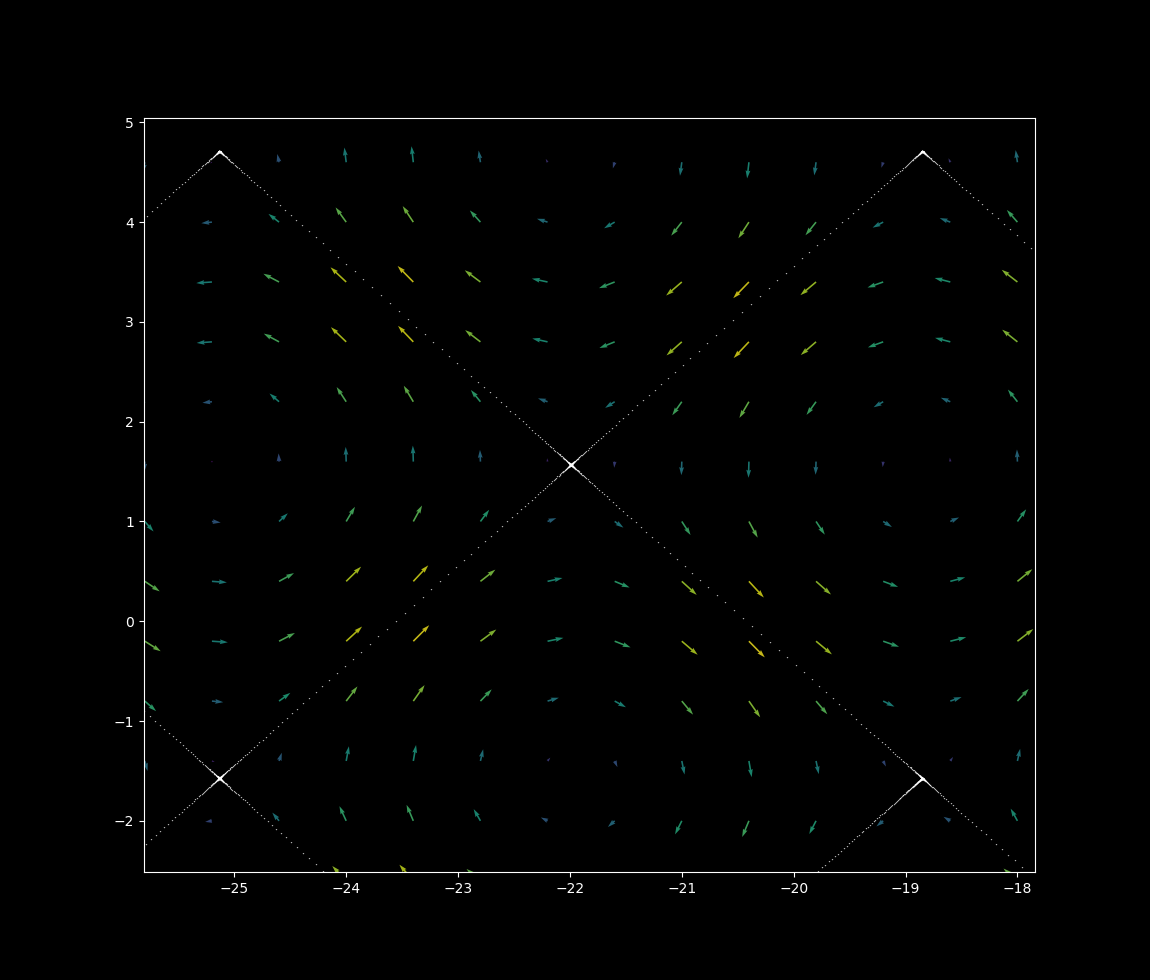
The differential system

\[\cfrac{dx}{dt} = a \cdot cos(y) \\ \cfrac{dy}{dt} = b \cdot sin(x) \tag{1}\label{eq1}\]

may be viewed using its vector map as follows:

Trajectories of particles obeying \eqref{eq1} may be observed with Euler’s method,

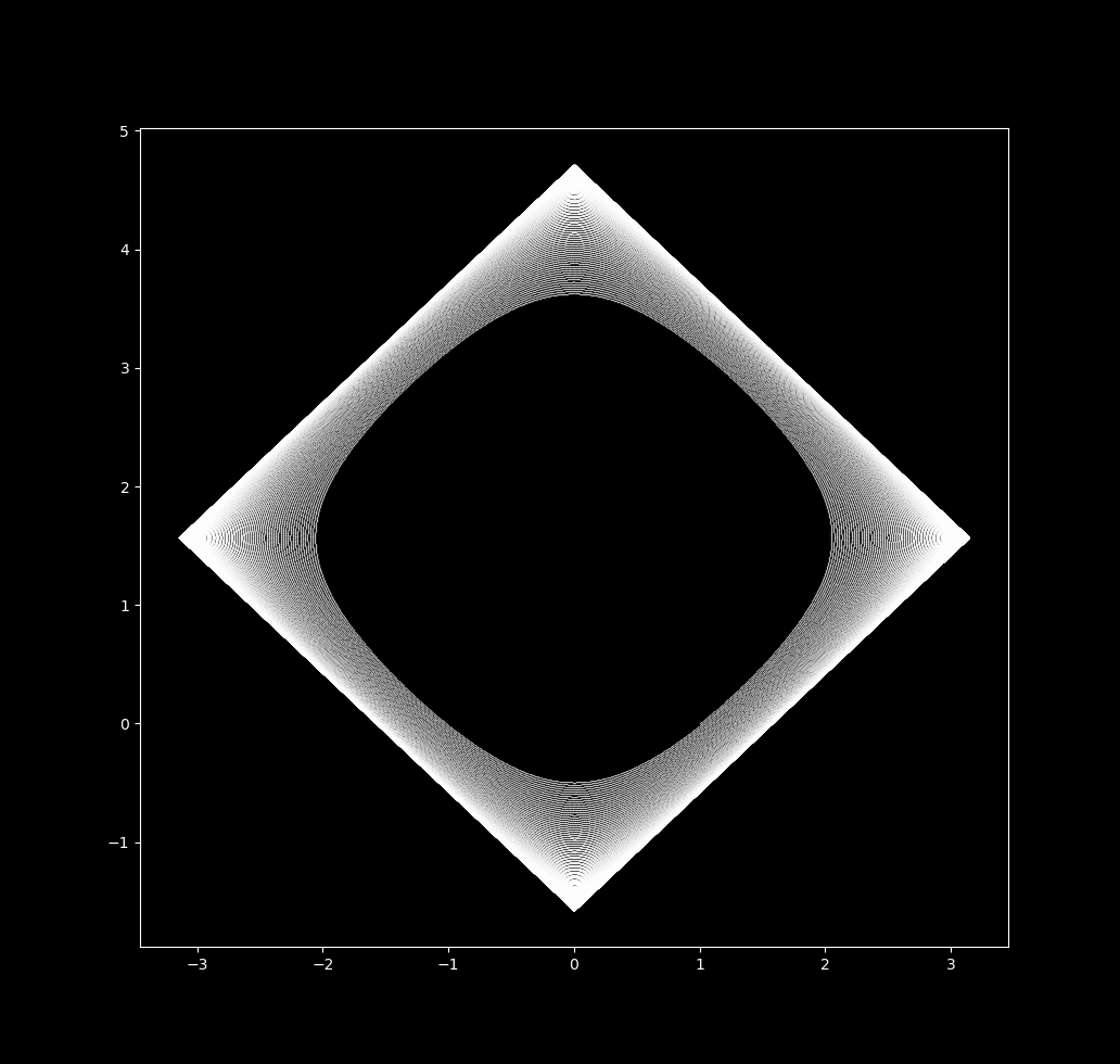
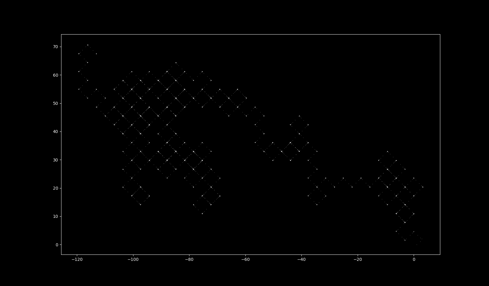
\[x_{n+1} = x_n + \cfrac{dx}{dt} \Delta t \\ y_{n+1} = y_n + \cfrac{dy}{dt} \Delta t \tag{2} \label{eq2}\]

\eqref{eq1} is an unbounded nonlinear two dimensional system. It is extremely sensitive to initial conditions for certain values of $\Delta t$. For example, take $\Delta t = 0.8$ and the starting $(x, y)$ coordinates to be $(1, 0)$. The following map is produced:

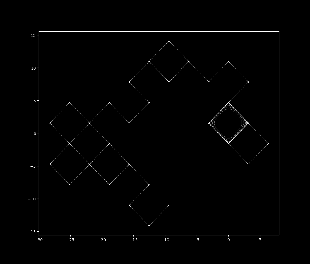
If the starting $x$ coordinate is shifted by a factor of one billionth (to 1.000000001), a completely different map is produced:

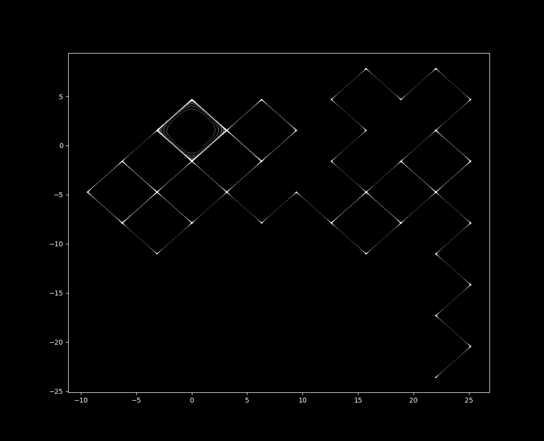
Animating the trajectory of both of these maps with $x_{01} = 1$ in red and $x_{02} = 1.000000001$ in blue, we have

Euler’s formula is used to (not very accurately) estimate the trajectory of unsolvable differential equations. Here it is employed with deliberately large values of delta_t in order to demonstrate a mapping that is not quite continuous but not a classic recurrence (discrete) mapping either.

This idea becomes clearer when the vector map is added to the trajectory. Observe how the particles are influenced by the vectors, as is the case for a continuous trajectory,

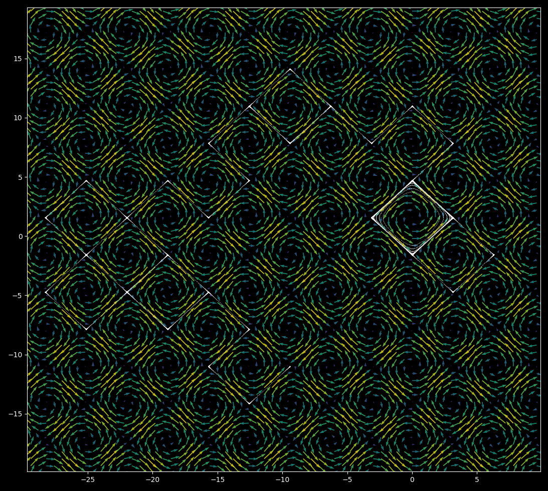
and that on close inspection there are gaps between successive iterations, as for a discrete recursive map

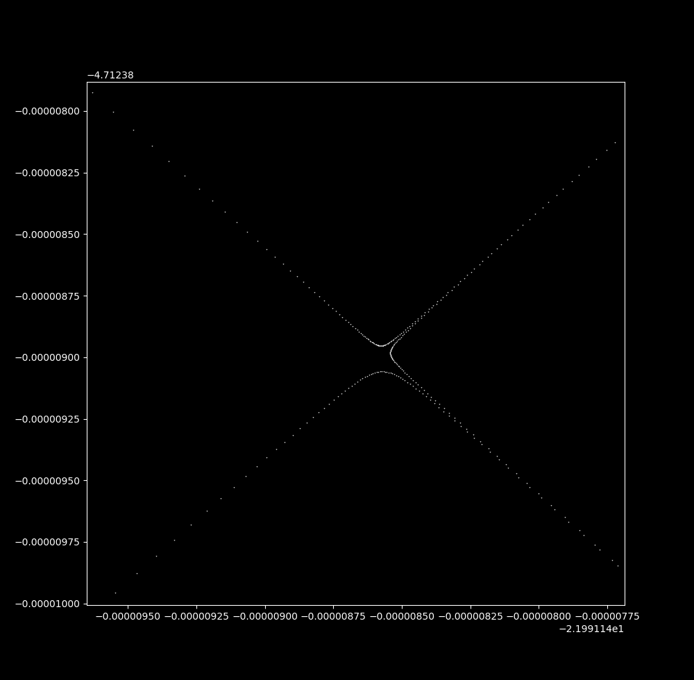
Systems of ordinary differential equations have one independent variable: time. This leads to all trajectories being unique. How is this grid map possible given that each vertex point seems to lead to multiple trajectories? The answer is that the trajectories get very close to each other but do not touch. At a smaller scale, an intersection of grids is revealed to not be an intersection at all.

\eqref{eq1} is an example of a chaotic mathematical system as it is deterministic but deeply unpredictable: small changes to the starting value of a chaotic system will lead to large changes in the output. These are also called aperiodic systems, because they never revisit previously visited points.

An aperiodic, unbounded map

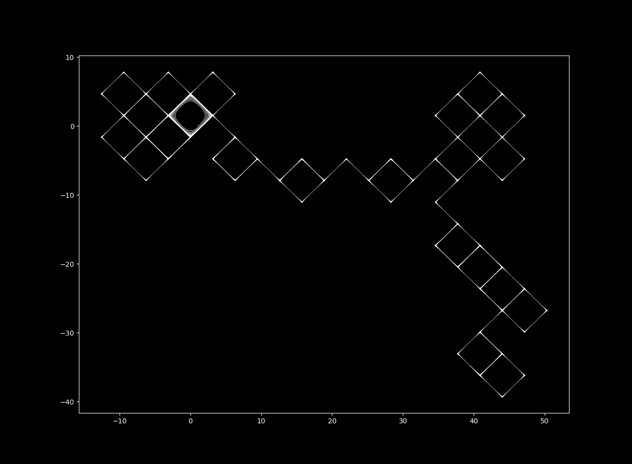
The grid map is an example of an aperiodic but unbounded trajectory. Aperiodic trajectories must cross each other if bounded, meaning that if one connects the iterations of a discontinuous map over time the connections must cross one another (for why this is, see here). But as the grid map is unbounded, a trajectory does not necessarily have to cross itself in this manner in order to be aperiodic. For larger $\Delta t$ values detailed below, the trajectory does indeed self-cross.

The grid map displays sensitivity to initial values typical of aperiodic maps, and although not bounded the trajectories head towards infinity very slowly.

The grid map is indistinguisheable from a random walk Brownian trajectory for some $\Delta t$

Imagine a ball with elastic collisions to sparse particles that flow in the vector map pattern, or else a ball moving smoothly that is only influenced by the vectors at discrete time intervals. Observe what happens with increases in the time step size:

$\Delta t = 0.05$

$\Delta t = 0.5$

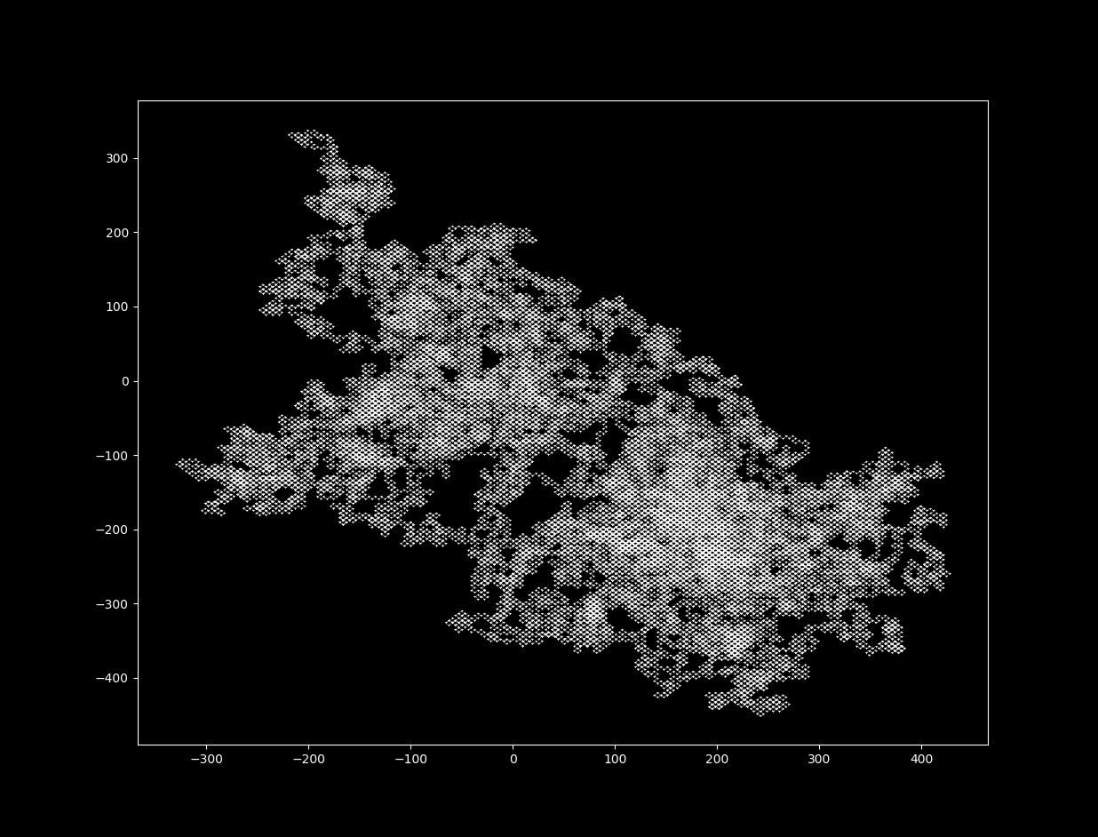
$\Delta t = 13$

$\Delta t = 15$

$\Delta t = 18$

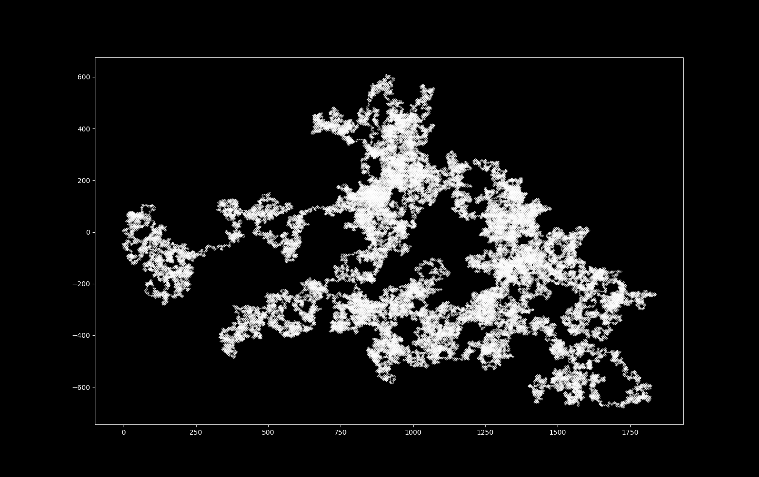
Which has a trajectory that is formed as follows

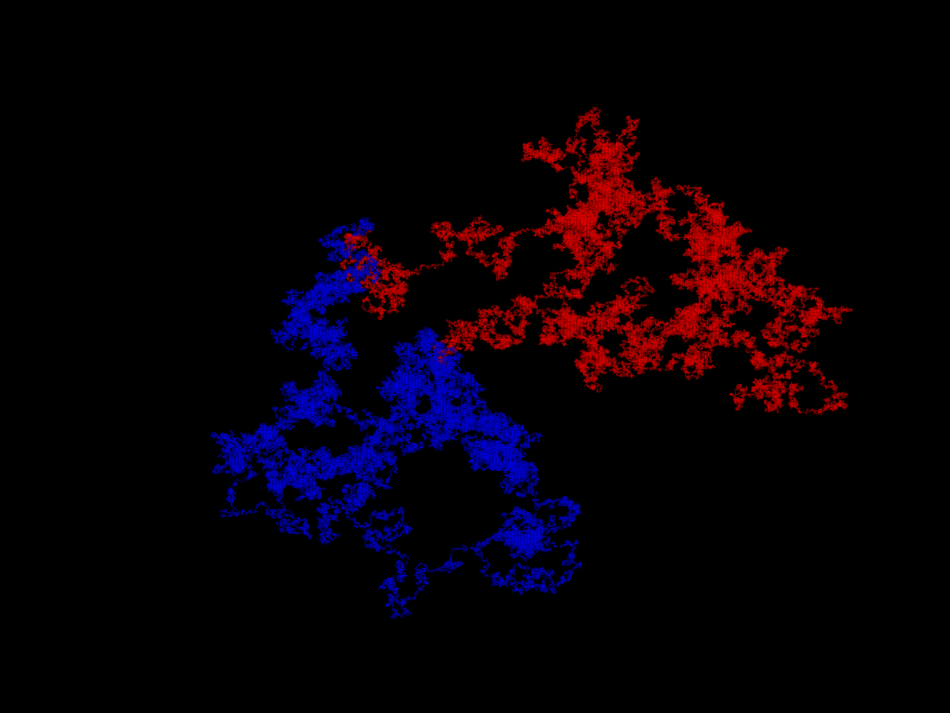
and still remains extremely sensitive to inital values ($x_0 = 1$ in red, $x_0 = 1.000000001$ in blue).

With increases in $\Delta t$, the map’s fractal dimension increases. It is impossible for 2-dimensional continuous differential equations to produce a strange (fractal) attractor, but it is possible for a 2D discrete system to do so. For more on this topic, see here.

At $\Delta t = 18$, the trajectory is indistinguisheable from random walk, which is often modelled mathematically by a system called a (Wiener process). This is not peculiar to the equation system \eqref{eq1} but is a feature of many nonlinear systems (see the logistic attractor or Clifford attractor pages) that are iterated discontinuously.

Why is this important? It means that real observations that are normally ascribed to a stochastic (usually linear) model are equally ascribable to deterministic nonlinear models. And this is important because once we have perfomed an inversion with respect to what can be ascribed to stochastic versus deterministic events, we can invert the reasoning on what is insignificant data (‘noise’) versus what is significant (‘signal’). What one normally thinks of as signal may actually be far less important to understanding an underlying physical process than what is considered noise.