Memory Models
Introduction
The ability to compress information from a sequence of tokens into one embedding in an efficient manner has a significant utility: we can use these embeddings to provide exended context to a model without increasing its inference computation. Extensive research has been performed on methods to reduce the amount of computation and memory required to train and perform inference on a model applied to $n$ tokens, and this problem has been particularly relevant to recent advances in code generation, mathematical problem solving, and other domains benefitting from chain-of-thought test-time compute scaling. In this paradigm, the performance of a model scales with the number of tokens one generates (before generating a final answer) such that inference compute and memory become significant bottlenecks.
On the compute side, transformers scale with $O(n^2)$ for $n$ tokens (assuming $K, V$ caching) making very long context window inference prohibitevly expensive unless one has access to large GPU clusters. This is true regardless of whether one uses a mixture of experts or attention innovations such as multi-headed latent attention, as these only introduce constant factors to the scaling complexity. Memory requirements are $O(n)$ during inference if $K, V$ caching is used and $O(n^2)$ during training as caching cannot be used as one must backpropegate across all activations.
Decreasing both memory and compute growth is an active area of current research, with most efforts aligned with attempts to use sub-quadratic complexity attention or attention alternatives. Here we take a different approach: our generative model is still $O(n^2)$ compute (and $O(n)$ memory if caching is implemented) for inference regardless of mixer or transformer use, but we provide embeddings representing entire sequences as inputs to that model in certain indices rather than only embeddings representing tokens. For the case where we have one encoder model and one decoder of a fixed length, the compute required is $O(n)$ with length (a slight abuse of notation as this is only valid up to the length $n_{ctx}^2$) as one simply uses more of the decoder’s embedding indices for sequences rather than tokens, and similarly the memory scaling is $O(1)$ again only up to $n_{ctx}^2$.
The idea of compressing input sequences into embeddings that take the place of transformer token embeddings is not new, and was explored in various forms (see particularly the recurrent memory transformer). Such models were shown to be able to perform simple information retrieval (needle-in-haystack style) on the compressed inputs but little more than that, and certainly do not retain most information of the input. The insight here is that as we have seen that transformers are quite inefficient with respect to capturing input information in encodings but masked mixers are not, we can use masked mixer encoders instead to greatly increase the amount of information that is stored in each embedding.
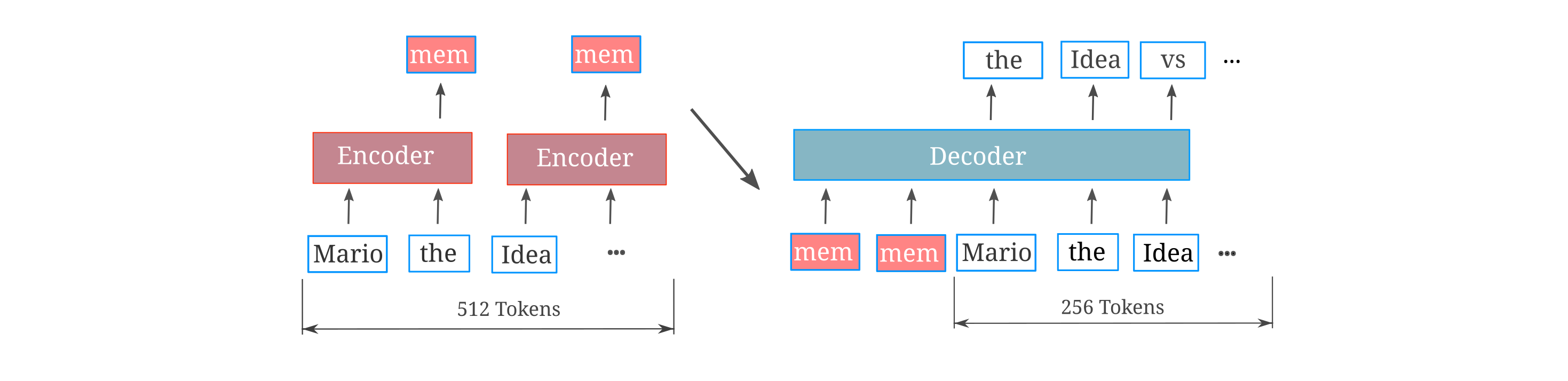
The architecture we will experiment with here is mostly similar to the embedding-augmented causal langauge model architecture implemented above, where we use the token dimension concatenation to maximize the number of embeddings we can provide to the decoder model. We begin by testing the ability of a memory embedding to provide information to allow for an increase in decoder causal modeling accuracy where this embedding is formed from all tokens in the sequence, both previous and future, which we refer to as an ‘oracle’ memory. For clarity, a transformer-based architecture used for such oracle memories is as follows:
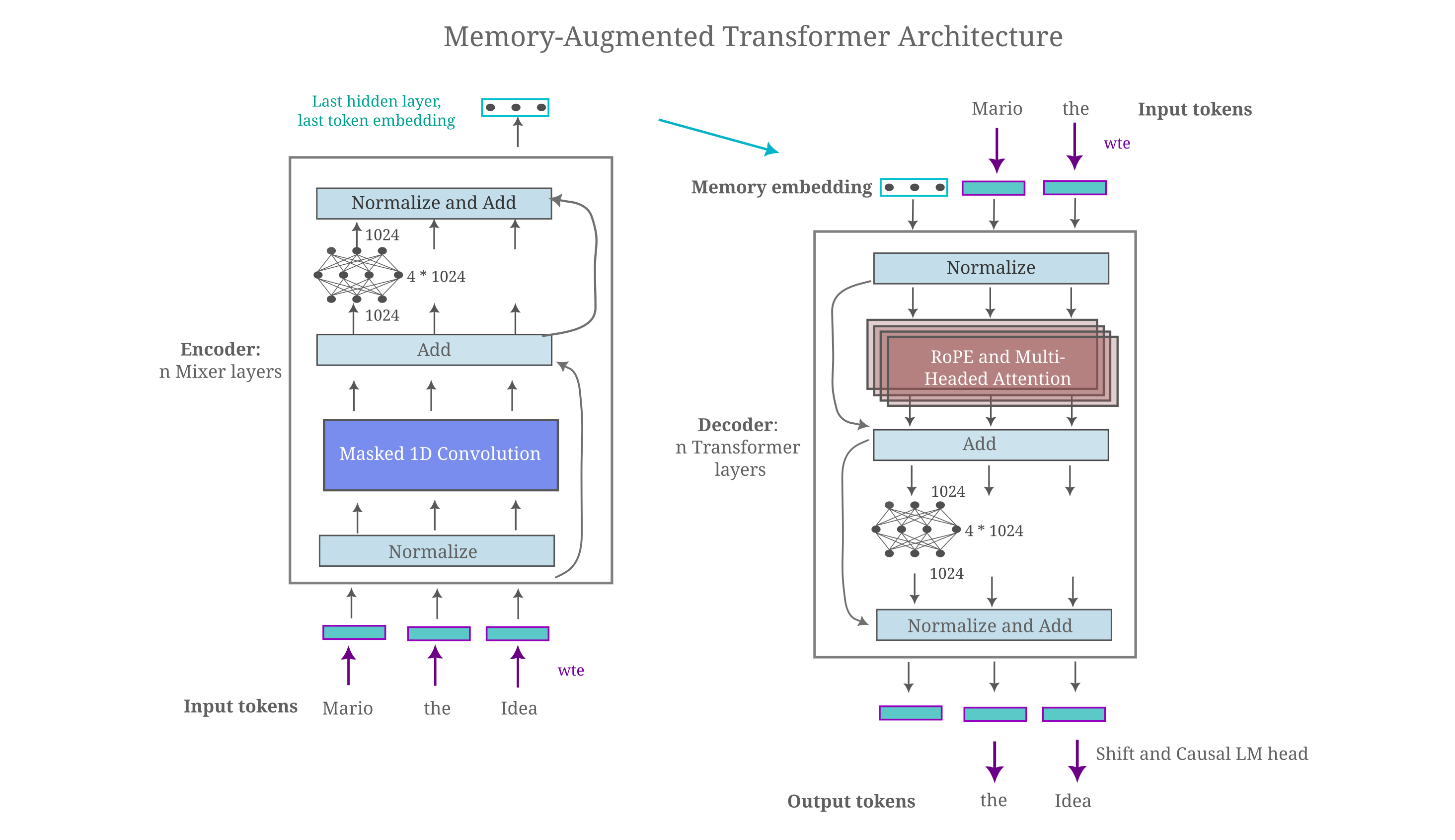
After testing the ability of oracle memories to capture necessary information of the input to effectively minimize causal language modeling loss, we then explore models where the memories are only of past tokens.
The notable difference between this architecture and the token concatenation-based autoencoder introduced above is that we not longer care about compressing the embedding fed from the encoder to decoder. This is because if one uses token concatenation, each token in the decoder is converted to a vector of dimension $d_m$ such that it is natural to supply the encoder’s embedding as a vector of that same dimension. This also allows us to provide embeddings of $n$ encoded text sequences as $n$ embeddings, taking the place of $n$ tokens of the decoder. It is clear to see that this is much more efficient in terms of decoder input space than embeding concatenation, and avoid sthe problems of input ambuguity present when performing linear combinations in the embedding dimension.
Oracle memories can be nearly perfect with limited training
The first question we can ask is as follows: can a causal decoder make use of the information present in an autoencoder’s embedding? Essentially the question we want to address here is whether the information present in the embedding passed from encoder to decoder in the autoencoding architecture (where all tokens are generated in one forward pass) is beneficial for the case where we train a causal decoder (where each forward pass yields only one token). We can test this by observing training efficiencies for a causal masked mixer and an embedding-augmented masked mixer, where the latter may be implemented by training an autoencoder, discarding the decoder, adding a causal decoder, and freezing the encoder’s parameters during training. To save memory and compute during training, one could simply save the embeddings generated by this autoencoder to storage and reference them when training and evaluating the decoder, but we choose the former implementation to avoid a significant storage overhead. From the figure below, we see that the answer is yes: including an autoencoder’s embedding leads to substantially lower cross-entropy loss for the causal decoder.
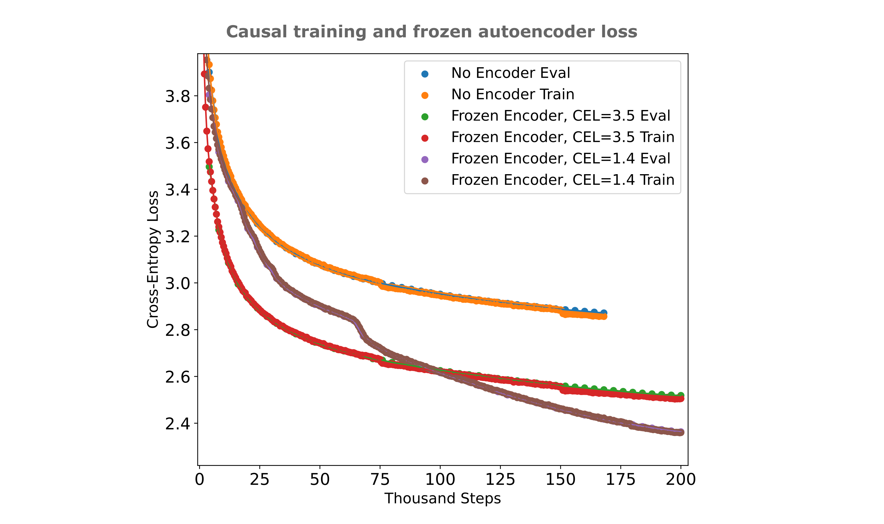
What makes a frozen encoder effective? Does an embedding from an autoencoder that has been trained more effectively (to a lower cross-entropy loss, that is) leads to more efficient training than using an embedding from a less-trained autoencoder, and are autoencoders more effective encoders than next-token-prediction (which we refer to as causal language model, CLM)-trained decoders?
From the figure below, we see that the answer to the first question is yes as there is a monotonic decrease in memory model loss as the autoencoder encoder’s loss decreases, although not to the degree such that a perfect encoder is capable of resulting in near-zero causal loss after our short training run (which is the case for optimized trainable encoders as we will shortly see). The latter observation likely indicates that the information learned during autoencoding (for a one-pass decoding) is fundamentally different from information that is useful for next token prediction.
The answer to the second question is that autoencoder encoders are indeed far more effective encoders than next token prediction-trained models, to such an extent that a rather poor autoencoder encoder (that only reaches a CEL of 3.5) far outperforms a causally trained model’s embedding that reaches a lower CEL of 2.6. Note that these models are all roughly compute-matched, such that one should accurately compare the causal embedding model with the most efficiently trained autoencoder. This is further illustration of the finding elsewhere that causal language models are not particularly effective information retention models, but rather tend to filter input information.
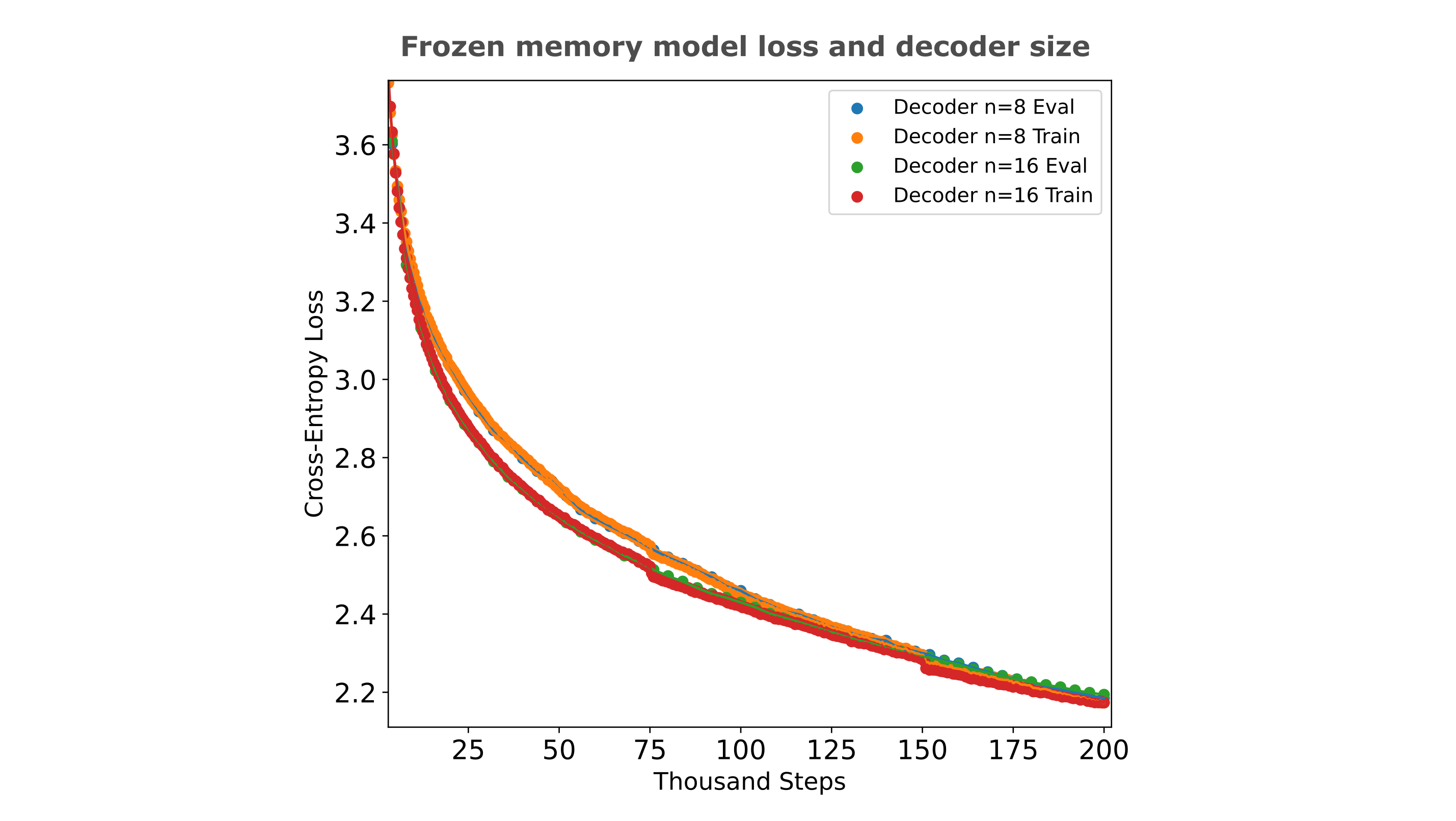
Given that we have seen more effective encoders resulting in lower causal decoder model loss, it may be assumed that the same would be true if one fixes the encoder and uses a more powerful decoder, say by doubling the number of layers from 8 to 16 (which for strictly causal decoders results in a drop in FineWeb evaluation loss from ~2.9 to ~2.65). Somewhat surprisingly, however, this is not the case: the same layer doubling in the decoder leads to no significant change in loss for a memory model given the optimial frozen (CEL=0.3) encoder used above. This counterintuitive result suggests that the decoder’s power is not a limiting factor for frozen memory models with effective encoders, but rather the number of samples passed to the model is more important.
Now that we have seen that casual decoders can indeed make use of encoded information, we can investigate the question of efficiency: is it better to train both encoder and causal decoder simultanously, or use an encoder from a previously-trained autoencoder and train the causal decoder separately? As shown in the left figure below, at least for a non-optimized encoder the answer is that training both simultaneously is far more efficient.
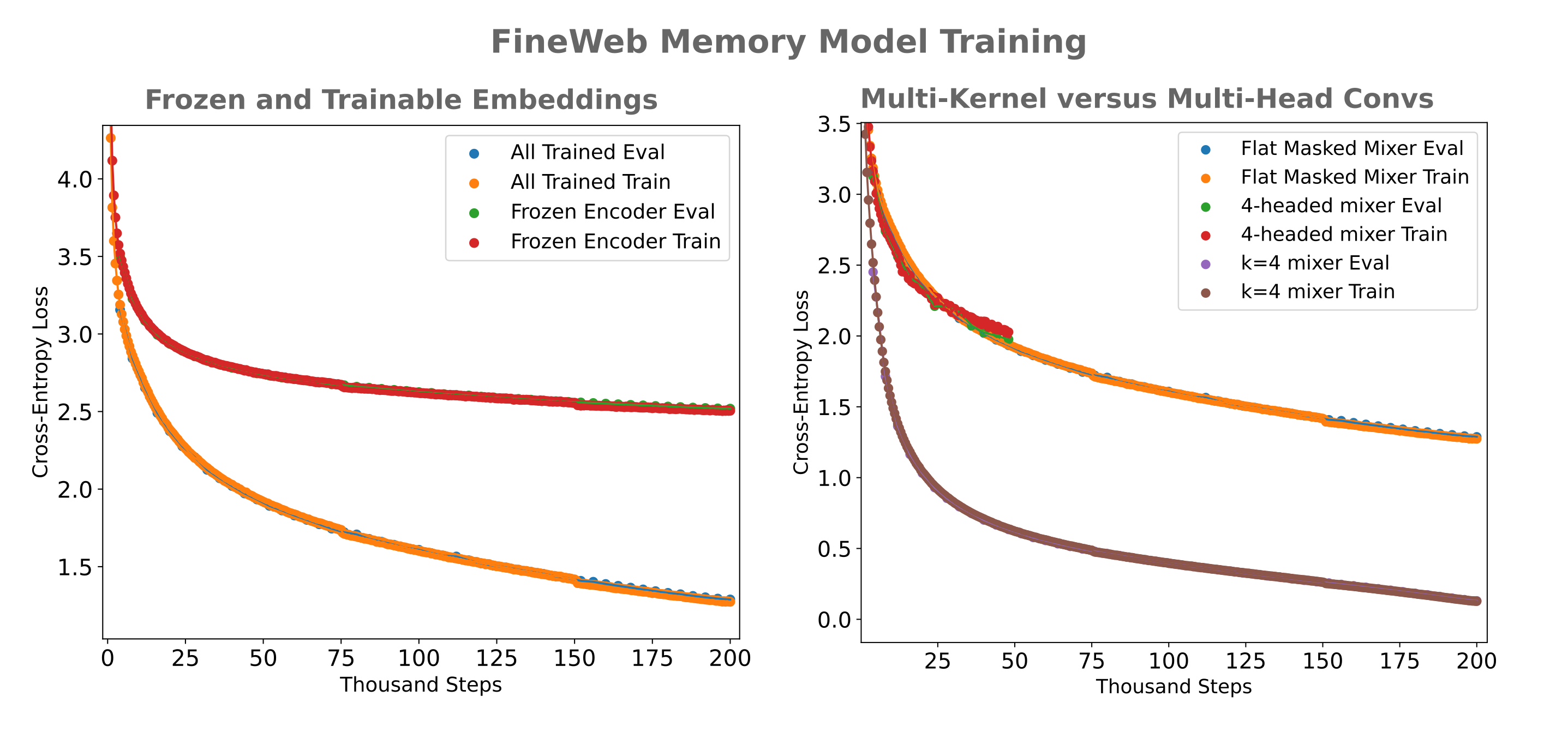
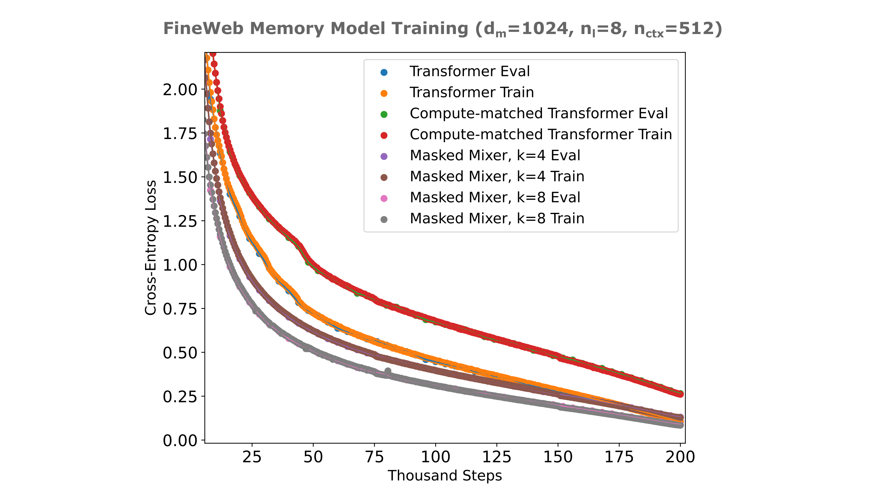
As is the case for memory models designed for information compression (ie with very small embeddings), a multi-headed mixer showed no benefit over the flat masked mixer early in its training run. Instead, we see a precipitous drop in cross-entropy loss when increasing the convolutional kernel to four (from one) to the point that our $d_m=1024$ memory model is able to effectively perform a $512 \to 1$ compression on token embeddings after training for half a day on two H100s with very little error resulting from this compression.
To conclude, the answer to our initial question in this section is yes: decoders (transformers or masked mixers) are certainly able to be trained to use information present in an encoder’s embedding,
Memory model training efficiency
Now that we have seen that decoders are indeed capable of learning to use practically all information present in an encoder, we can proceed with training memory models wherre encoders store information from previous tokens, not the token to be predicted.
A little reflection can convince one that if it were efficiently trainable, the use of such memory embeddings would be extremely useful both for increasing a model’s effective context window without increasing its inference computation as well as for cases where one would want to cache a model’s previous state as is common in multi-turn conversation or agentic workflows.
Thus the question remains whether or not a memory model is actually efficiently trainable, with an upper bound being the per-step loss achieved by ‘full-context’ models, meaning models that do not separate the input into chunks and form embeddings of these chunks but train on the entire input at once. We start by training relatively small memory models in which both encoder and decoder are trainable.
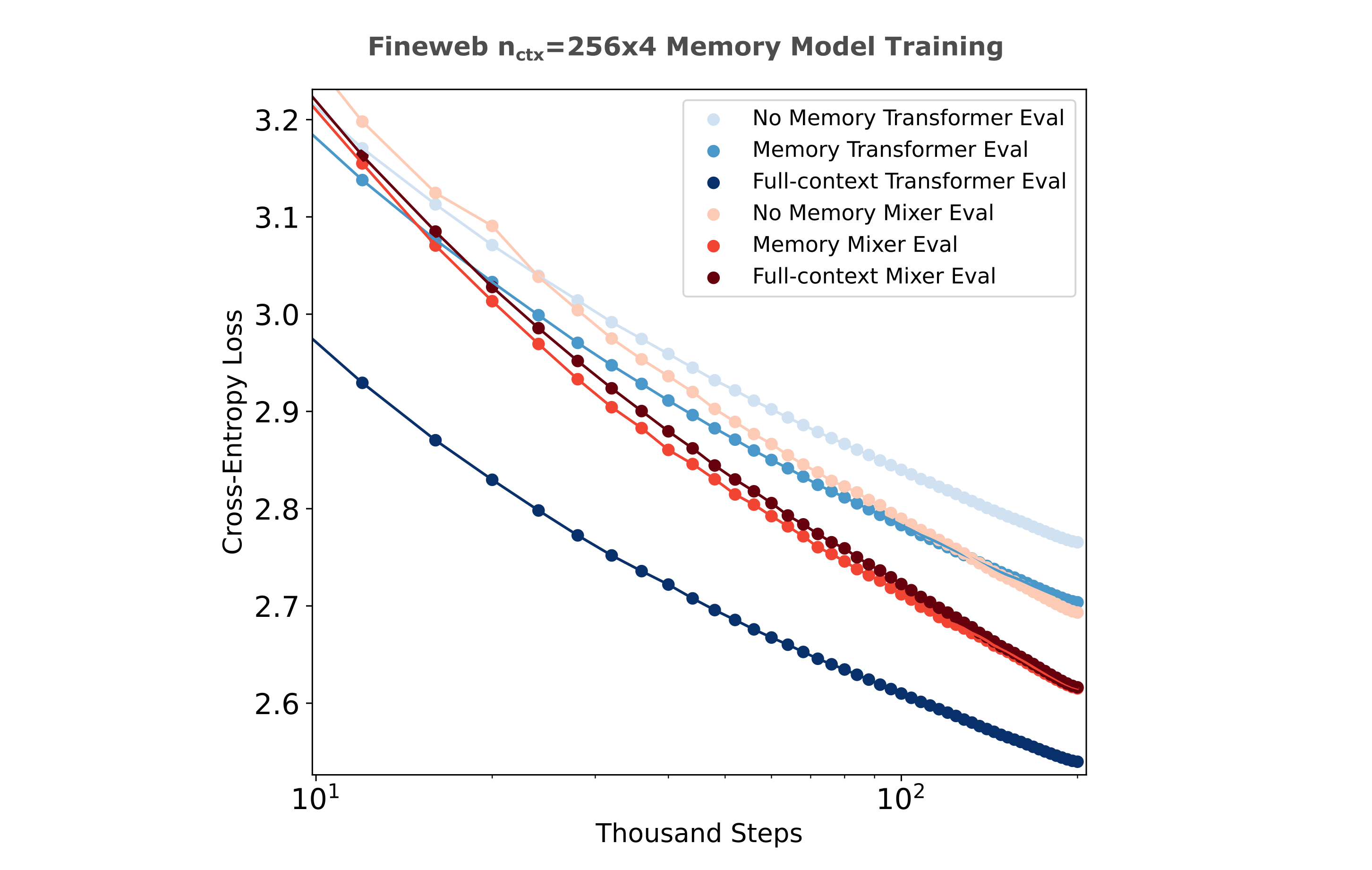
The experimental setup to address this question is as follows: we first obtain tokenized inputs of a certain length (here 1024 total tokens, potentially including padding) and then divide these into four chunks of 256 tokens each. Our encoder then forms embeddings of the first three chunks, and the decoder uses either zero (for the first chunk), one (for the second), two (for the third chunk) or three previous embeddings (for the fourth chunk) as it predicts each next token in that chunk. We compare this memory model training efficiency to the same architecture but with no memory embeddings added as well as full-context models all trained on the same dataset (full-context models of course do not use chunked inputs).
We use smaller encoders than decoders ($d_m/2$ of the decoder to be precise) in order to make the memory models more similar to the full-context models in terms of memory and compute required per training step than is the case for full-size encoders, at least to within around 20% or so the throughput.
In the following figure (note the semilog axes), observe that transformers and masked mixers are both substantially benefitted by the addition of memory embeddings as expected. What is more surprising is that the memory mixer is nearly identical in per-step training efficiency to the full-context model albeit with a ~25% lower throughput. The full-context model uses right instead of left padding as mixers don’t use attention masks (left-padded training is much less efficient for full-context but not memory models).
This is not the case for transformers, however, such that the full-context version of that model remains substantially more efficient to train than the memory-augmented version. The per-step loss difference between full-context transformer and memory mixer halves as training proceeds, making it likely with more training the memory mixer would equal or surpass the full-context transformer in terms of loss at a given training step. In the following figure, each model is trained on $128 * 1024 * 200000 \approx 26*10^9$ tokens.
It may be wondered whether it is beneficial to fix the positions of memory embeddings and token embeddings or else allow the indices of the start of token embeddings to vary. The difference between the fixed-position and variable-position embedding implementation may be depicted as follows:
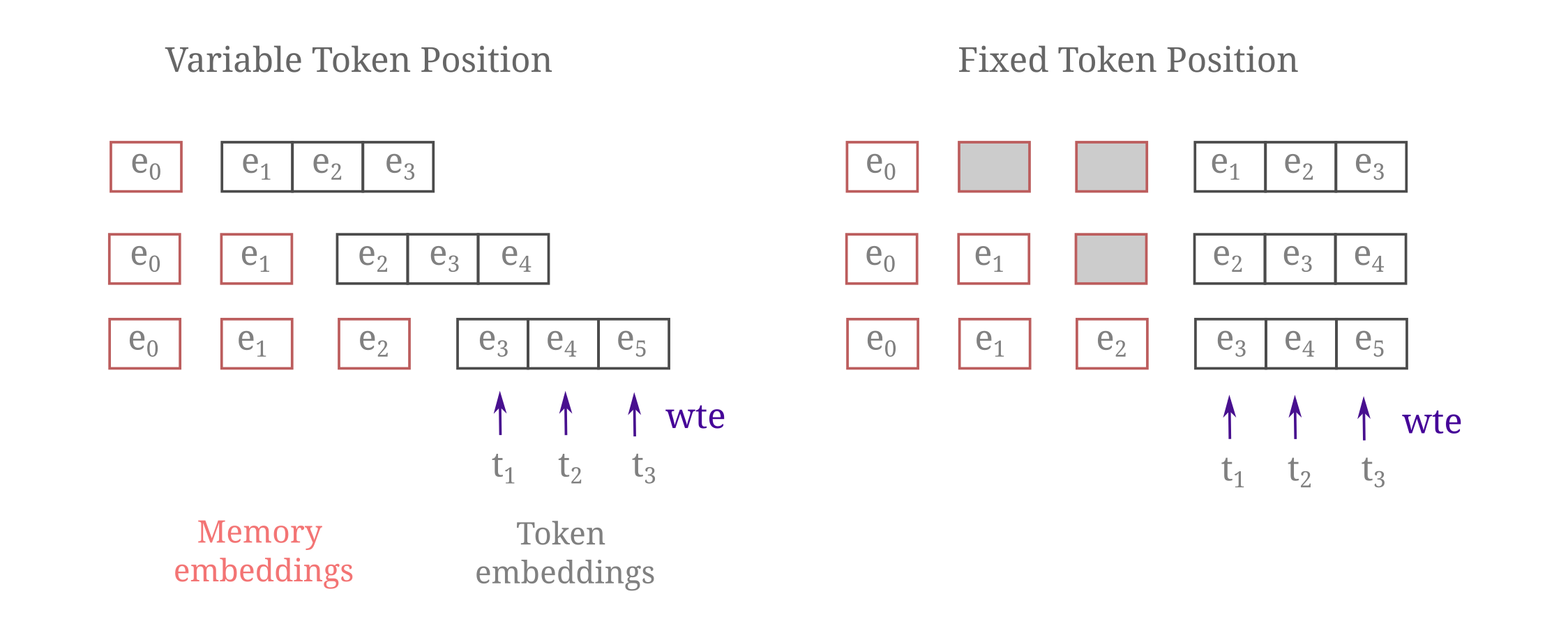
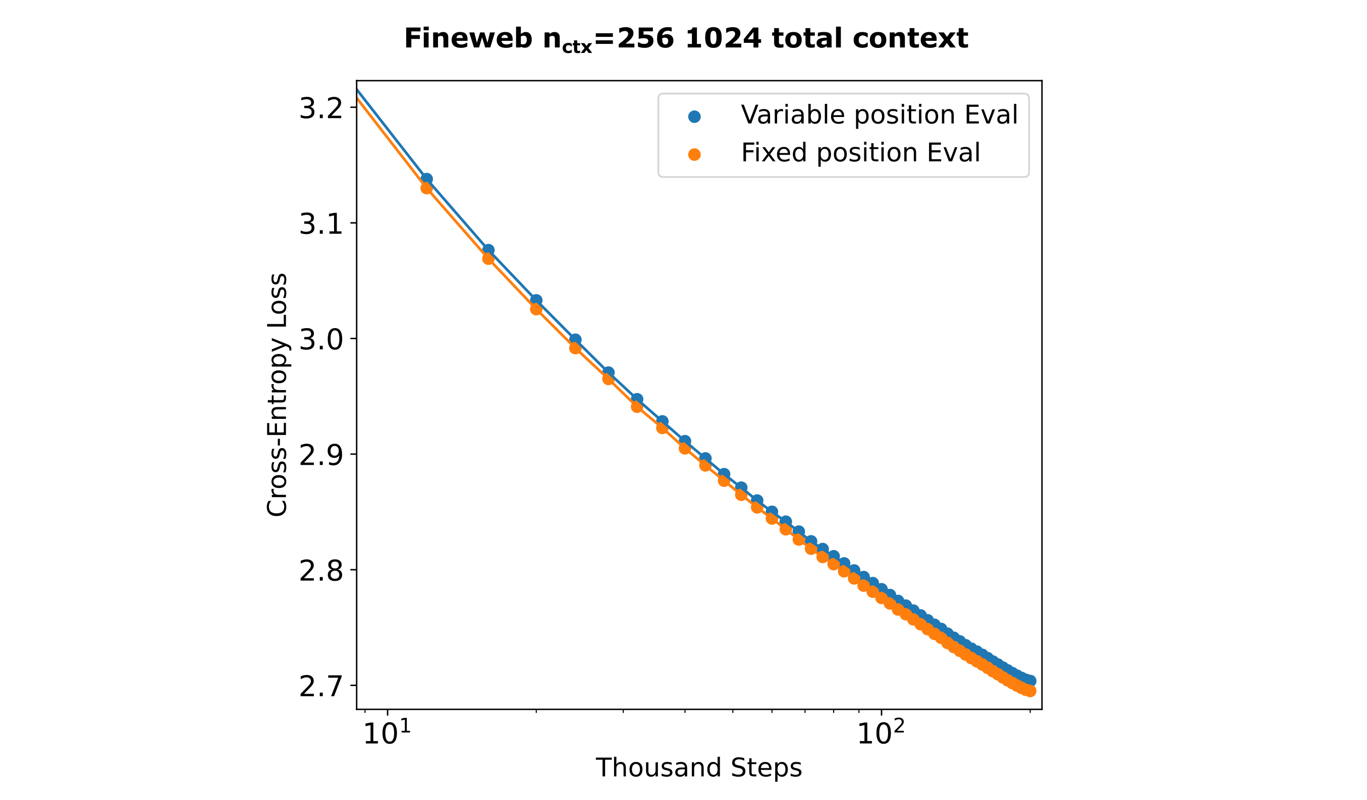
Masked mixers effectively use fixed, absolute positional encodings such that is is natural to use fixed-position embeddings. But as this is not the case for transformers, such that it is useful to compare the training efficiencies between fixed and variable position embeddings. As shown in the following figure, there is a rather small increase in efficiency using fixed positional encodings for transformers.
A separation between encoder and decoder allows for efficient training
It may also be wondered how these encoder-decoder memory models compare with decoder-only-style memory models with respect to training efficiency. A notable example of this is the recurrent memory transformer architecture in which a decoder model reserves one or more embeddings as memory ‘tokens’. For causal language modeling, this means that these decoders are tasked with both encoding (in the sense of storing information in the memory embeddings) as well as decoding, in the sense of using embeddings of tokens as well as sequences of tokens to generate individual tokens.
To show the difference between the encoder-decoder memory models as defined above (which we can think of as ‘parallel’ memory models) and recurrent memory models, the following diagram illustrates how each model type processes inputs of up to three chunks.
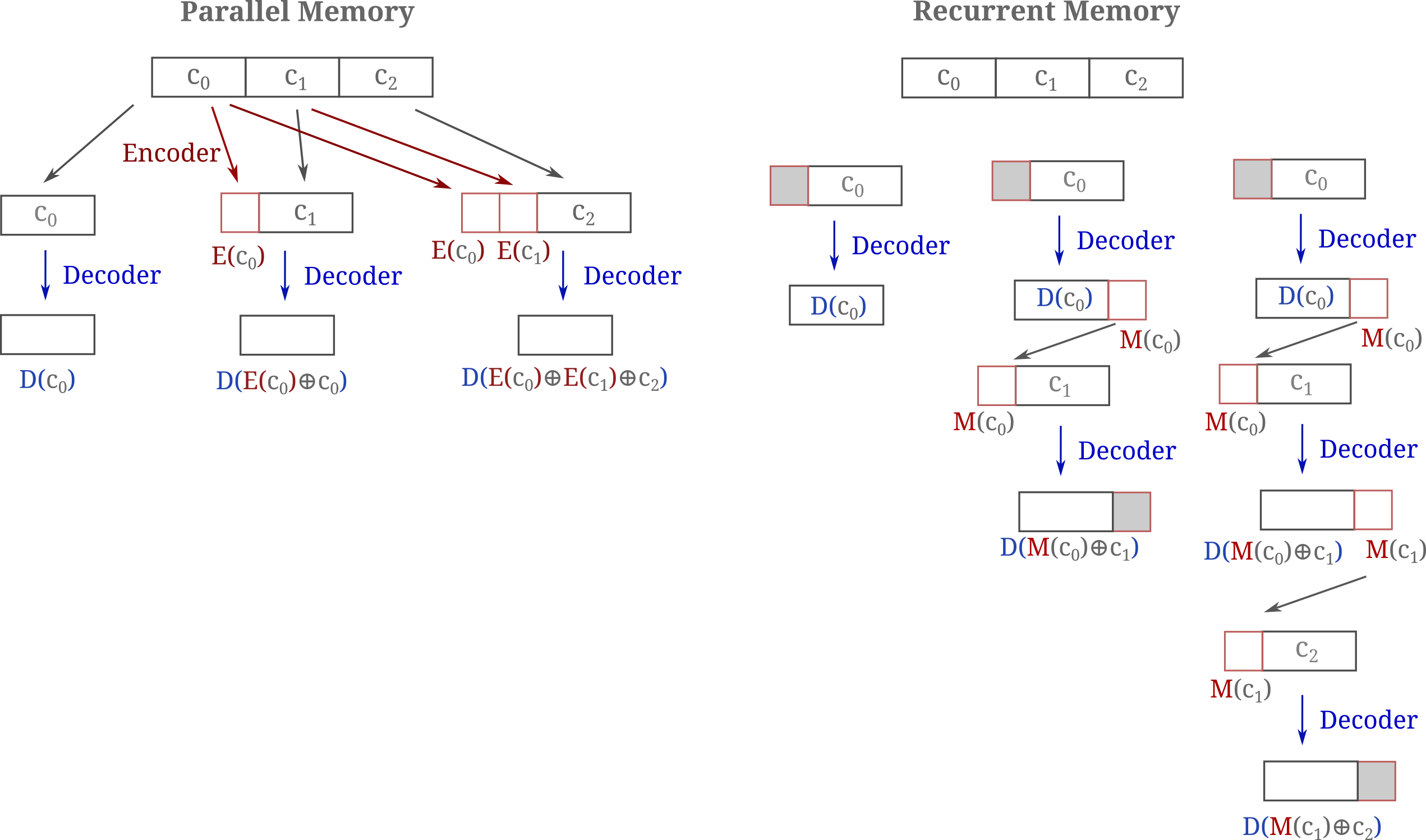
It is apparent that the encoder-decoder memory model exhibits a number of notably beneficial features compared to the decoder-only recurrent model both for training and inference. If both encoder and decoder are trainable, the total memory would be approximately equivalent to the recurrent model if the encoder were smaller than the decoder but the encoding can occur in parallel, avoiding the high sequential computational cost of back-propegation through time. In a similar manner, using parallel encoders also allows one to avoid the known difficulties associated with normalizing gradients accross many decoder segments typical of BPTT and recurrent memory transformers in particular. The same parallelizations are possible during inference, meaning that a long prompt may be processed much more quickly using the parellelizable memory model than the recurrent version.
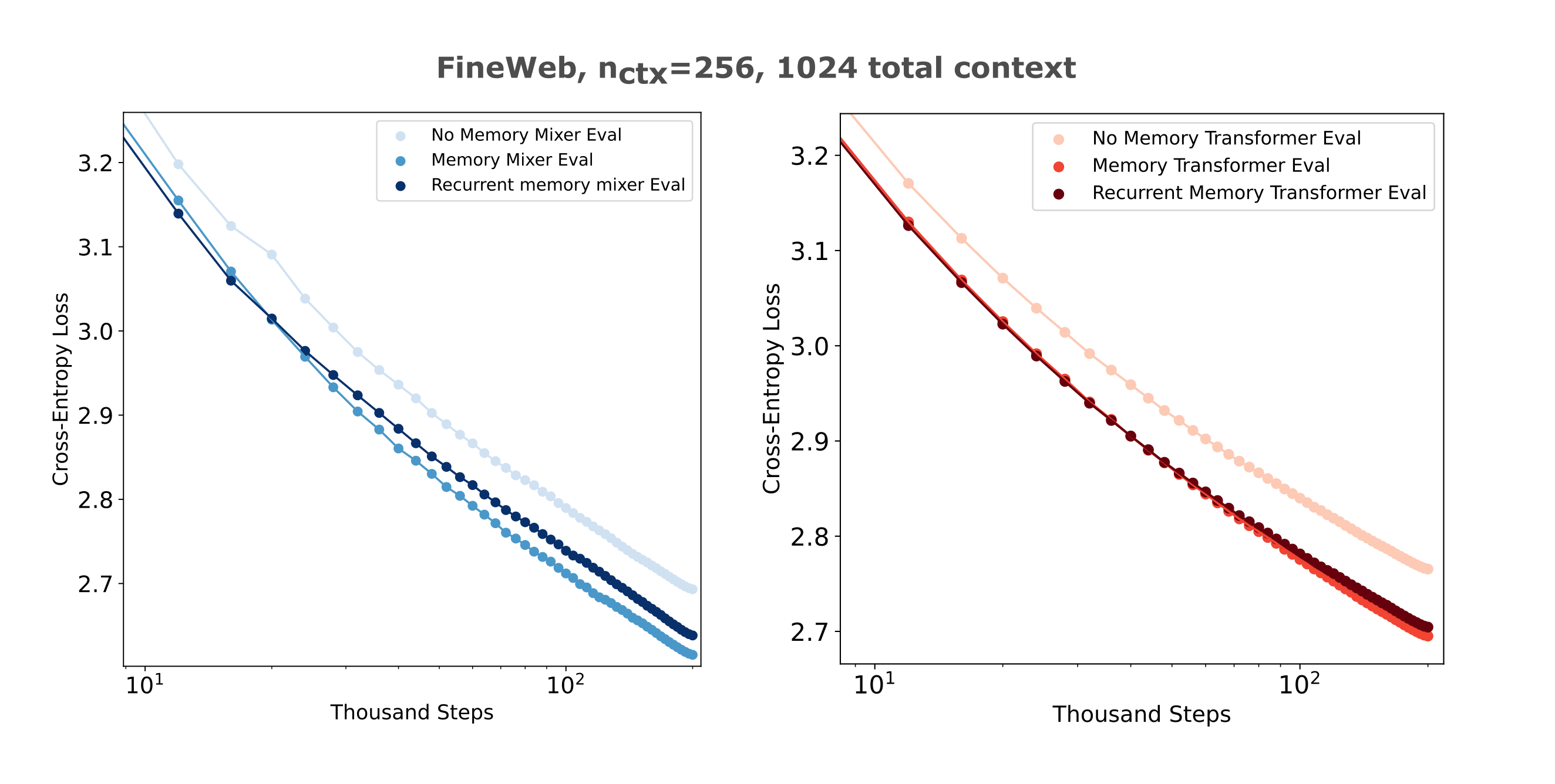
We test the training efficiency of parallel and recurrent memory models by comparing losses achieved on FineWeb inputs of up to 1024 total tokens with chunk sizes of 256 tokens, meaning up to three parallel memory tokens or a depth-four decoder stack for the recurrent model. We use one memory embedding for the recurrent model and perform back-propegation through time for the entire recurrence. In the figure below, we see that parellelized memory models are slightly more efficiently trainable in this paradigm, but that this effect is rather subtle and in the case of transformers likely not significant. The difference in transformer versus masked mixer losses per step are mostly accounted for by superior performance mixers exhibit for small-context (here 256 tokens) training windows.
If the memory models contain trainable encoders, these two architectures are very similar in memory and compute requirements for a given input and model size. This is because these models form gradients on all $n$ tokens of their extended context, which occurs for RMTs via back-propegation through time and for memory models via gradients on encoders. In the case of RMTs, it was shown to be necessary to perform this back-progegation through time in order to maintain training efficiency, and additionally other approaches that only back-propegate in local chunks (ie transformer-xl) exhibit worse performance.
Recalling that recurrent memory models combine encoder and decoder tasks into one architectural unit, this is not particularly surpising: clearly training an encoder is not efficient if one does not backpropegate an encoder’s gradients to model blocks on token indices that are actually required for information retention. Separating encoders from decoders would be expected to largely ameliorate this issue: instead, we can train an encoder first on all necessary token chunks and then use this model to form the memory embeddings that may be used to train the decoder without requiring gradient flow to the encoder. The fundamental idea here is that one may separate the encoding (information-saving) function from the decoding (information-discriminating) function in order to achieve very large memory savings during training.
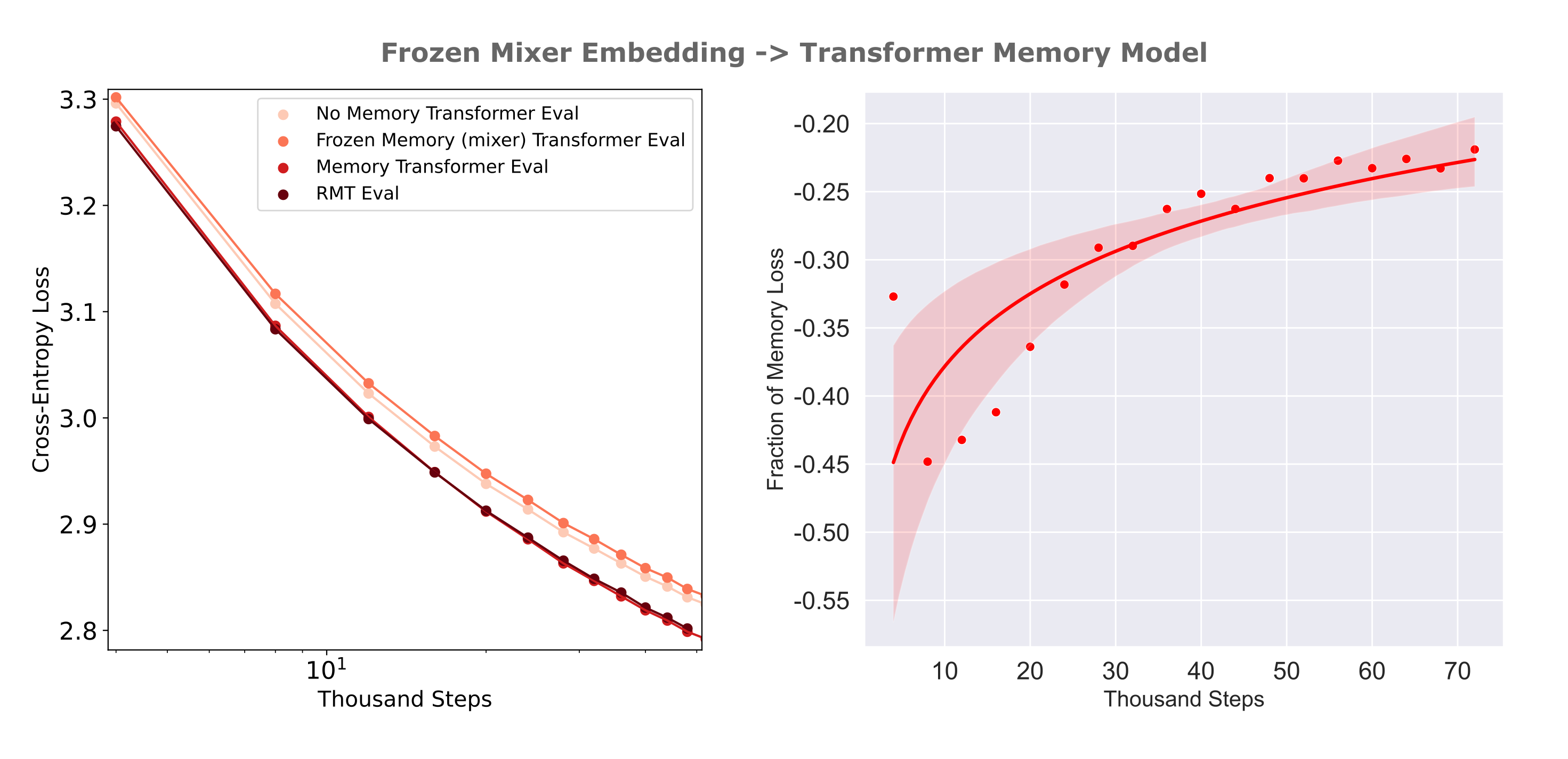
Is a memory model with a frozen encoder efficiently triainable? It would not be of much use to train using a frozen encoder if the decoder was not able to learn to use the encoder’s information efficiently in the first place. We can test this by comparing per-step losses of frozen encoder models to no-memory and trainable encoder-based memory models. The following figure (left) shows the training losses achieved using a frozen encoder with an architecture matched to the memory model decoder where both encoders achieve an autoencoder CEL of <0.3 on 512 tokens.
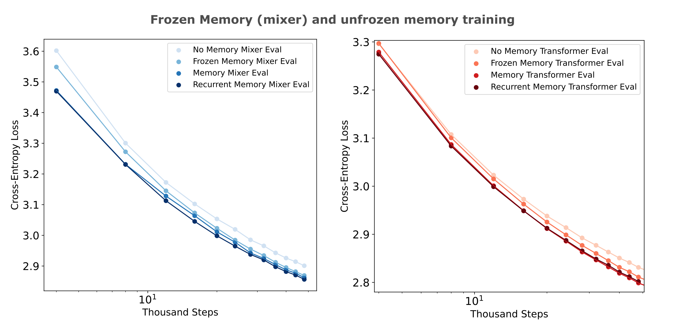
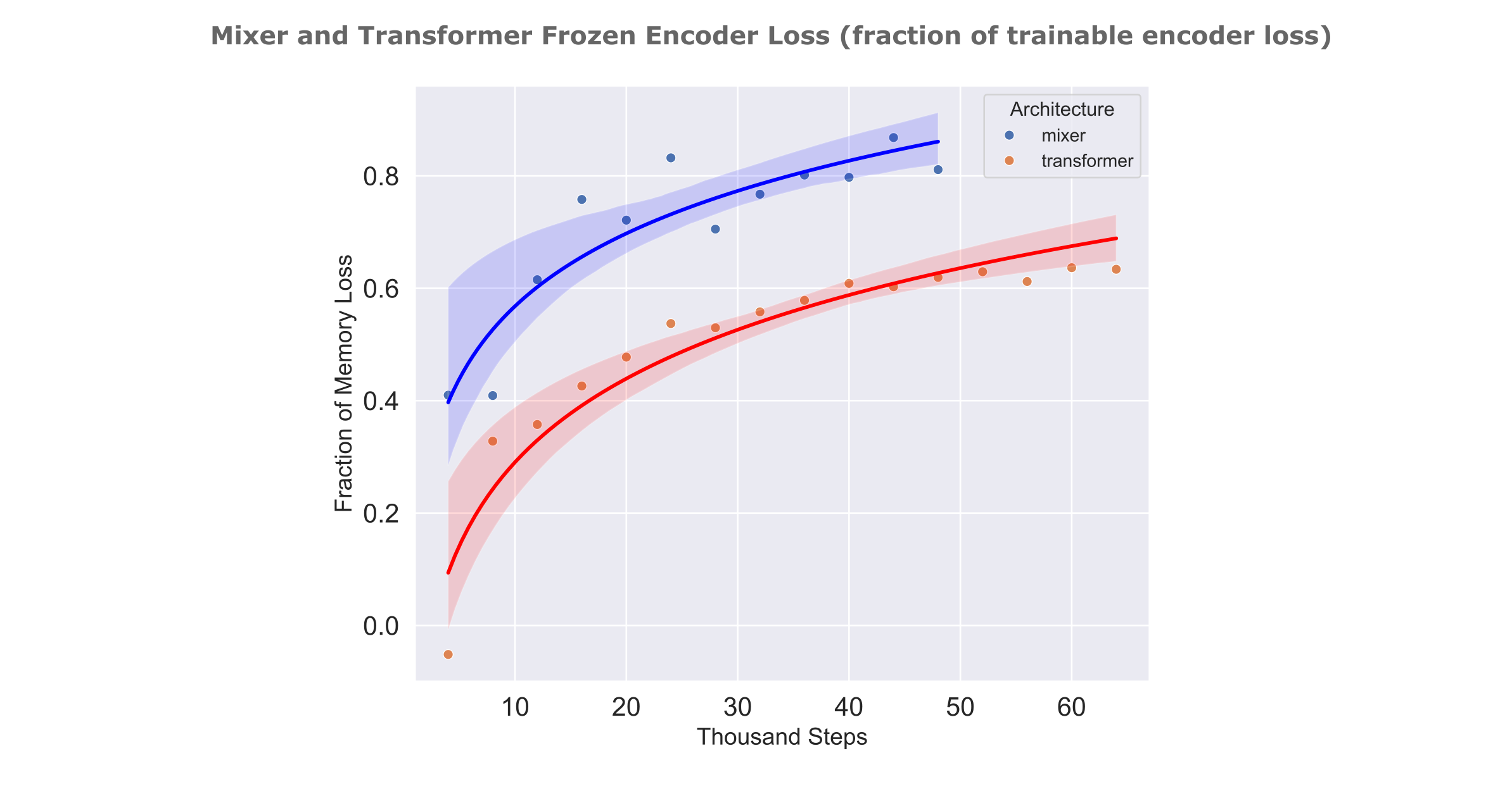
To display the differences between frozen and unfrozen memory model encoder training efficiencies more effectively, the right panel shows the proportion of memory loss (1.0 being equal to the memory models, 0.0 being equal to the loss of no-memory model at each step) achieved by mixer and transformer frozen memory models. For both architectures, we see that the difference between frozen and trainable memory encoder decreases as training proceeds, but it is also apparent that mixers are more readily capable of using frozen encoder information compared to transformers. This is notably not due to the encoder itself, as the transformer encoder used here achieved a slightly lower evaluation cross-entropy loss ($\Bbb L =0.289$) compared to the mixer encoder ($ \Bbb L = 0.292$) on the same dataset.
As we have seen in the text compression work that even trainable encoders are much more efficiently trainable if their architecture matches that of the decoder (meaning that we pair mixer encoders with mixer decoders and transformer encoders with transformer decoders), it may be wondered if a similar phenomenon would here such that the transformer decoder would be less capable of using the information present in the mixer’s embedding. We find that there is actually an increase in per-step loss for a transformer memory model if it is given the mixer embedding compared to a model with no memory at all, suggesting that this transformer decoder is more or less comopletely incapable of using a frozen mixer encoder’s information, at least early in training.
How much embedding information can causal decoders learn to use?
So far we have assessed memory embedding use by causal decoders by training these models on datasets like FineWeb and FineMath in order to be able to form an approximation of the training properties on large and diverse corpora typical of frontier model pretraining. It is evident, however, that modeling this dataset does not actually require much information from previous tokens, at least not for the training scales we investigate (10 to 30 billion tokens in total). This can be appreciated by observing that continued training of a memoryless model results in these models attaining the same loss as memory models achieve with somewhat less training samples, and that naturally models with a context window of 256 (without memory) need to be trained on more tokens to match memory models a total context of 1024 with memory compared to models with a context window of 512 without and 2048 with memory.
What this means is that our training tests are not very effective measures of memory use by the decoder, as one would expect for only a little information to be required for the above observations. We can test this expectation directly by observing the training characteristics of a memory model in which the decoder is a frozen clm-trained decoder, as we know that these models contain a relatively small amount of input information across their entire context window. The results of this experiment are as expected: swapping out a clm-trained encoder for the autoencoder-trained encoder does not result in significant decreases in memory model training efficiency [add fig].
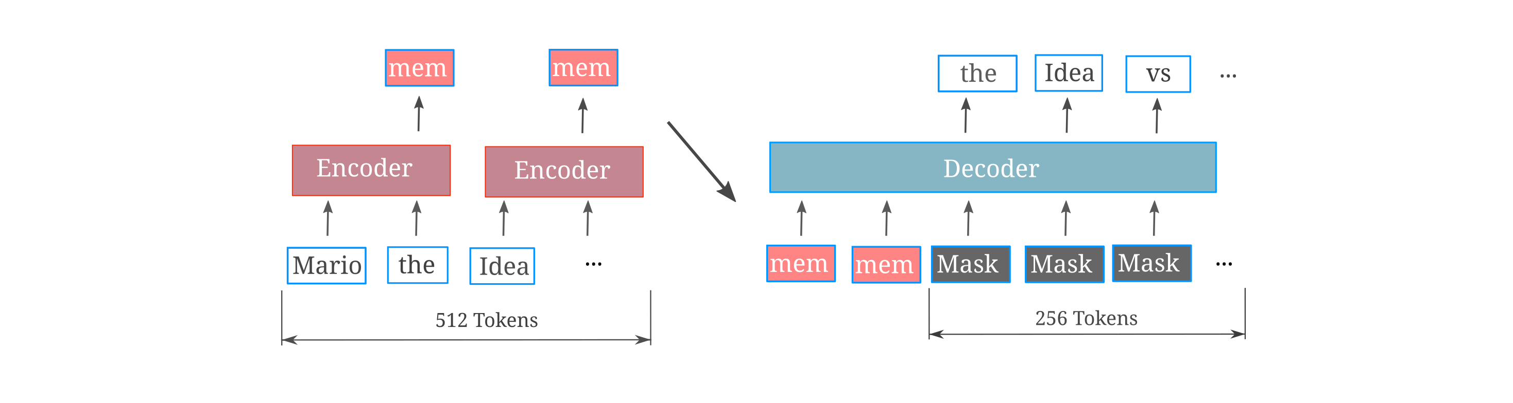
This provides motivation for a more effective test of memory useage for decoders. What we want is the ability to determine whether or not a causal decoder can make use of all the information in each memory encoding, and one way to test this is to train memory models on an input copy task. Here, given a certain number of tokens (say 512) the task is to train the model to be able to copy these tokens causally. Here the input tokens to be copied are given in the first 512 indices, such that the decoder’s third and fourth chunk must use only the information present in memory embeddings to perform this copy task. We mask the loss on the first two chunks so that the model is trained strictly to copy next tokens for which there can exist information in the embedding to perform perfect copying. A diagram of this experimental setting is given below, for the case where a 512-length input is copied (for a total of 1024 tokens) and a 256-context window memory model is applied to four chunks of this embedding. This depiction corresponds to the model’s configuration for the third chunk.
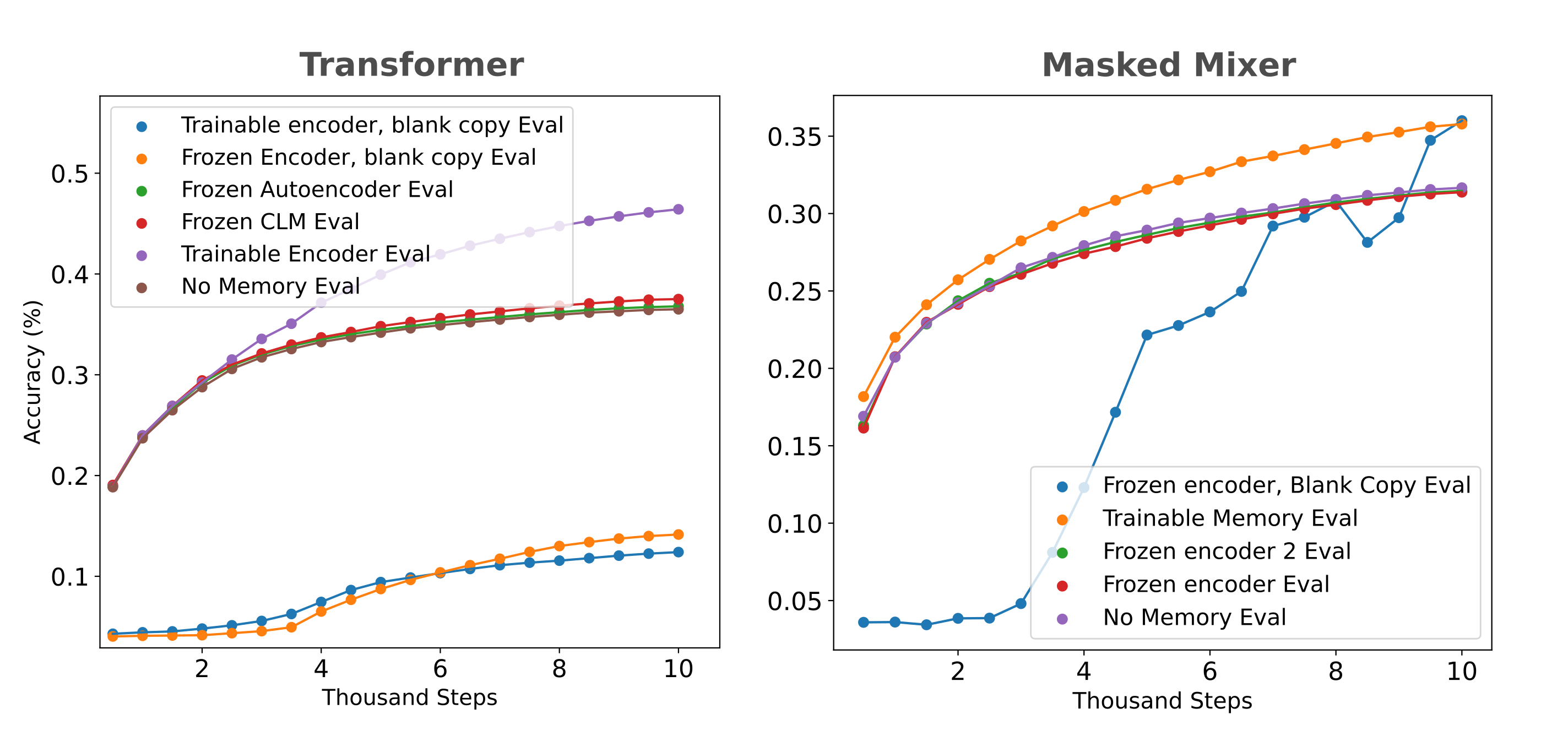
We train memory models on this copy task where copied inputs are sampled from the FineWeb with pad tokens added as necessary such that not all inputs actually contain 512 nonpad tokens copied. Models are evaluated on hold-out samples that contain strictly 512 non-pad tokens, or in other words a full-context copy task, and the results for mixer and transformer-based memory models ($d_m=512$) are given below:
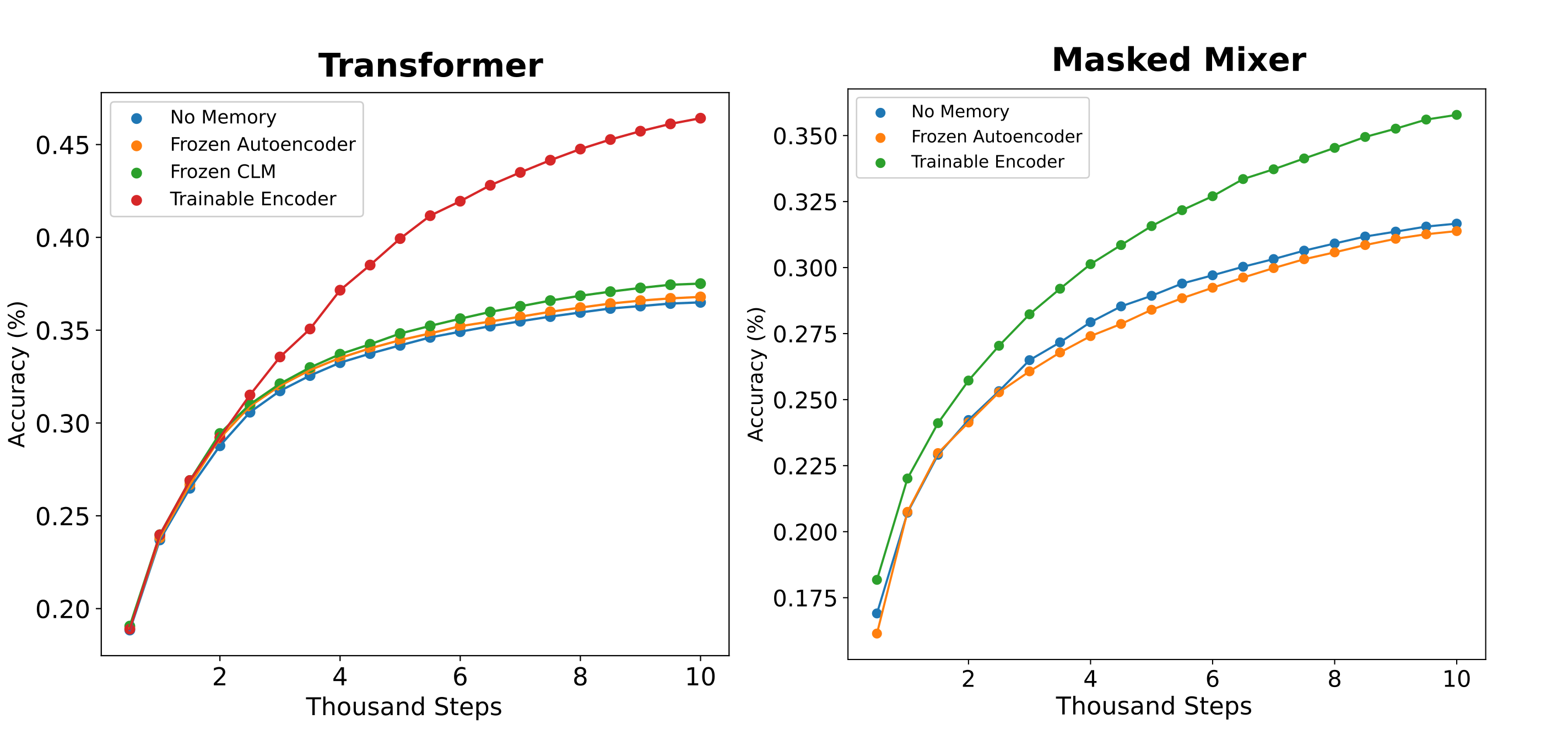
The results are unexpected: although one might predict that a frozen causal embedding would not result in substantial increases in copy accuracy due to the low informational content of these models’ embeddings, the frozen autoencoders obtain very low loss (corresponding to >95% autoencoding accuracy for their context windows) but curiously are also unable to inform the causal decoder to any significant degree. For mixers, autoencoders of multiple sizes were tested to ensure that the problem was not a malformed model or other model-specific implementation detail.
Why would a causal decoder be unable to use the information present in a rich embedding? There are three primary differences between the autoencoder architecture and the copy memory task: firstly that more than one embedding is fed to the decoder (and an unrolled projection is not applied), secondly that the decoder is causal in the sense that it predicts next rather than current tokens, and finally that the decoder receives both embedding information as well as current token information instead of only embedding information.
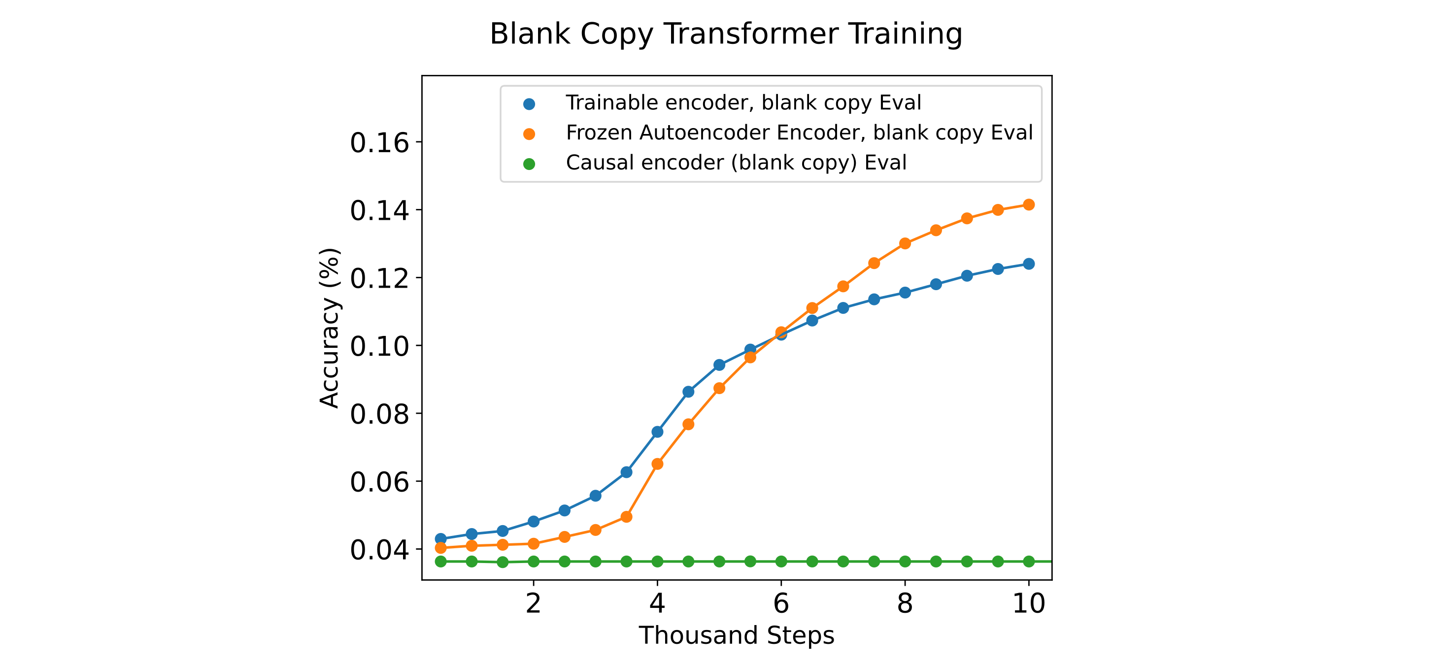
The third difference may be considered to be most likely to be the case: causality would not be expected to be an issue in itself as the embedding should be processable in any orientation, and using two embeddings rather than one should make things easier for the decoder rather than harder. We can test this hypothesis by removing the input ids from the copy (which we call a ‘blank copy’) such that all input information must originate from the embeddings, and repeat the copy training experiments.
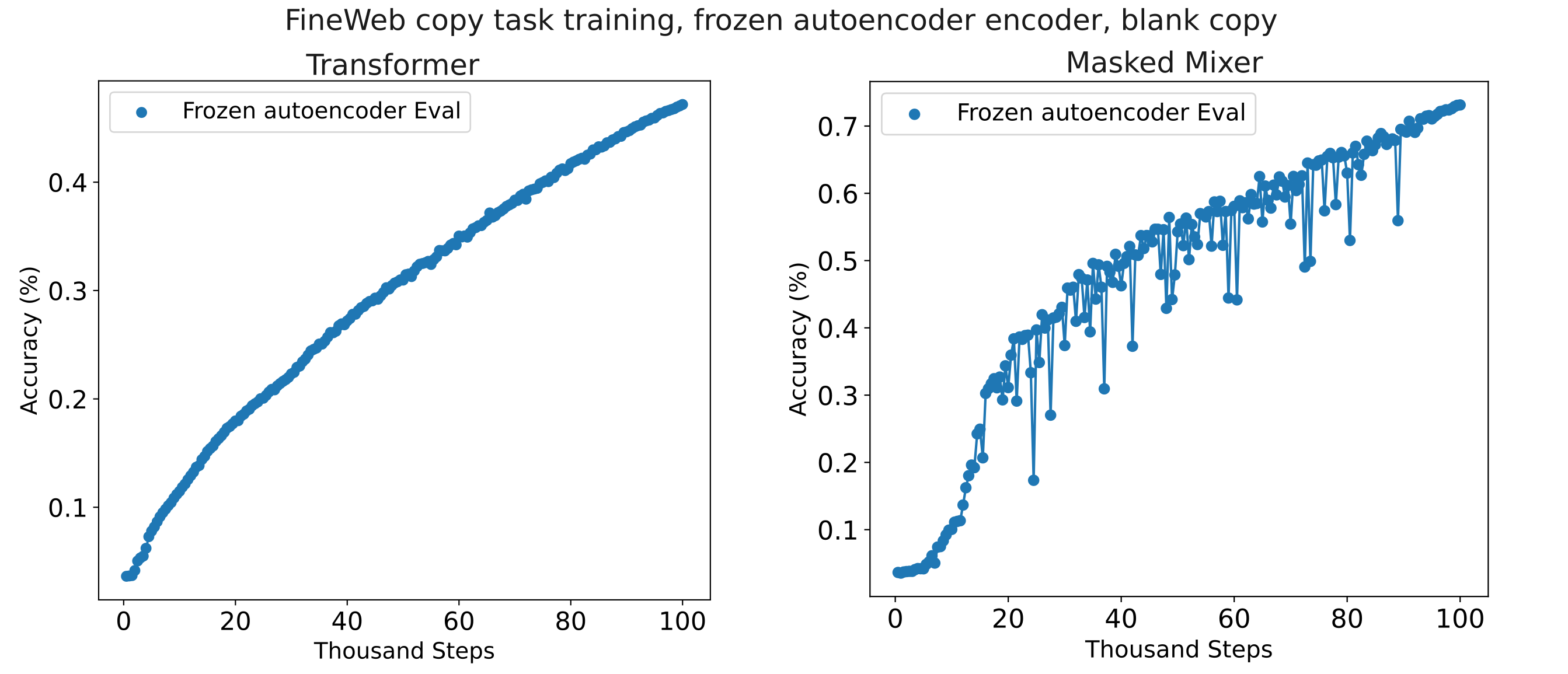
We find that masked mixers do indeed learn to use the information in the embedding if copy tokens are not supplied, resulting in higher accuracy than the trainable encoder memory model at the end of our relatively short training.
In longer training runs, we find that blank-copy trained masked mixer and transformer memory models (with frozen encoders) are both able to outperform the same models when the copy tokens are supplied to the decoder. All this suggests that it is indeed the presence of the tokens given to the decoder that inhibits the use of frozen encoder information during training by the decoder. One may hypothesize that the ability to decode a frozen encoder’s embedding is relatively difficult compared to next token prediction at the start of training, so the decoder learns to ignore the embedding as a result.
We may test the above hypothesis a few different ways. One method could be to first train a memory model on the copy task (with decoder tokens supplied) with a trainable encoder until that model exhibits high accuracy before then swapping in a frozen encoder and retraining for the same task. Another is to initialize a memory model with a frozen (pretrained) encoder, train the decoder without copy tokens provided (ie trained as a blank copy), and then train with copy tokens provided. The first of these approaches is essentially a transfer learning approach where the decoder’s ability to use trainable memory embeddings upon copy training is the basis for being able to use frozen memory embeddings, and the second is a curriculum learning approach whereby one single model (frozen autoencoder encoder and trainable decoder) first learns to use the information present in the encoder’s embeddings and then learns to use this information in combination with the information present in the tokens fed to the decoder.
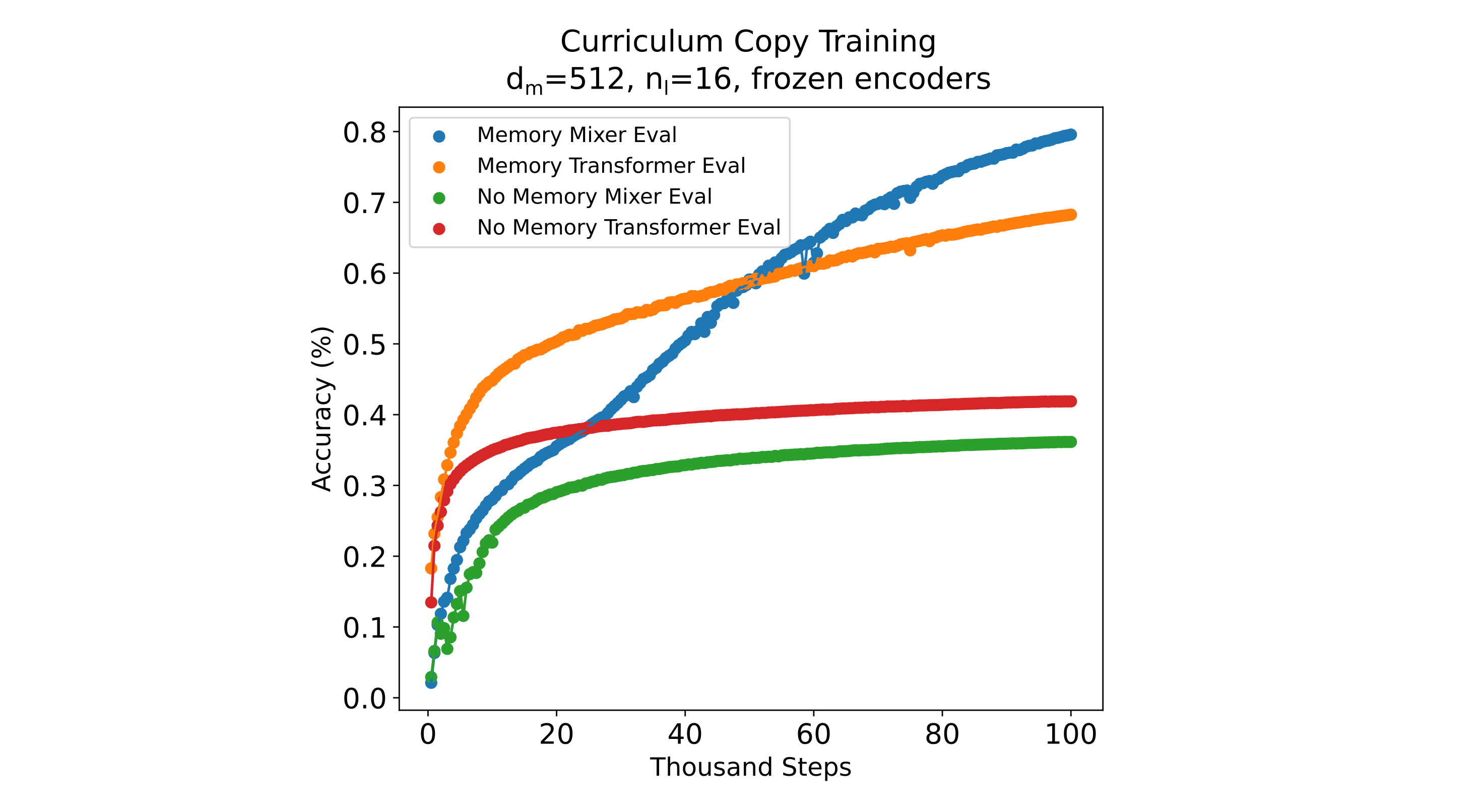
It may be guessed that the second method would be more efficient if token information were easier to decode than compressed embeddings, and the first if the converse is true. Previous results suggest that decoders generally find decoding tokens easier than decoding compressed embeddings, so we proceed with this approach. To restate, the aproach is to first train a high-fidelity autoencoder, then freeze the encoder and train a memory model (in this case $n_{ctx}=256$ per chunk, four chunks) while masking the copied tokens to the decoder (ie blank copy training), and finally load the weights to this model, keep the encoder frozen, and train to copy with tokens exposed to the decoder. For a negative control, we repeat this prcedure but do not supply embeddings in the final training procedure to observe the ability of the decoder to learn to predict each next token without memory embeddings supplied. As can be seen in the following figure this curriculum learning procedure results in effective use of (frozen autoencoder) memory embeddings for both transformer and masked mixer, and indeed they learn to copy more effectively than the embedding-only copy models. Once again the masked mixer is somewhat better at decoding the frozen memory embeddings, which is not due to the embedding fidelity itself (both transformer and mixer autoencoders achieve <0.03 CEL loss on this context window).
Can the same curriculum be applied to causal pretrained models? The answer appears to be no, at least not easily: as shown in the following figure, memory models train very poorly on frozen causal encoders when decoder tokens are not provided.
Pretrained Causal Decoders and Memory
So far we have investigated the introduction of memory embeddings into decoders that are initialized from scratch and then trained to make use of these memories. The next question to address is whether a pretrained decoder could also make use of memory embeddings as well, and we start by investigating this question with respect to trainable encoders and decoders.
To start with, we train a relatively small encoder ($d_m=512, n_l=16, h=4$ transformer) with a 1 billion parameter Llama 3.2, both using the 128k-size Llama 3.2 tokenizer, with a relatively small learning rate $5*10^{-6}$ with AdamW (larger learning rates were observed to result in divergence for this configuration). We observe a rapid increase in copy accuracy at the start of training (notice the large loss gap between the untrained model and the first checkpoint), followed by a far more gradual increase in copy accuracy as training proceeds.
We can hypothesize that this is the result of the decoder learning to filter our most of the information from the (as-yet) untrained encoder model as that embedding is likely very different from any token embedding the decoder has learned to process, rather than actual memory use learning. This may be tested by training the same model where the encodings are randomly assigned and not from trained models (ie there is no actual memory at all), whereupon we see a near-identical loss gap early in training.
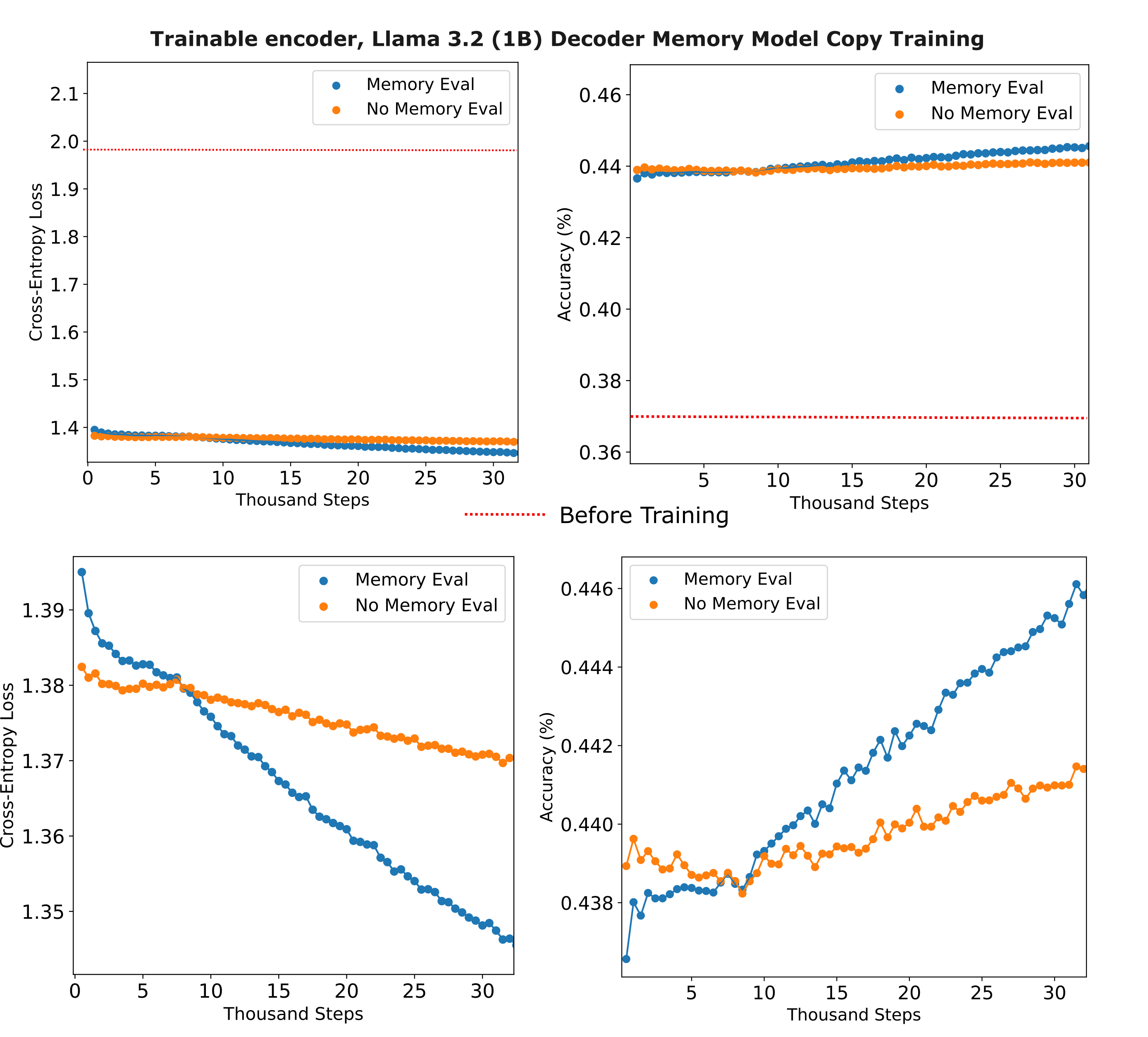
That said, it is clear that the decoder is able to extract useful information from the memory encoding: in the lower plots on the figure above, we see that the memory model quickly outstrips the copy accuracy of the memoryless model by around a thousand training steps (sixteen thousand samples).
Why do pretrained models train relatively inefficiently as memory model decoders compared to untrained decoders? We observe a 1% increase in copy accuracy after 30k steps of training a Llama 1B decoder with a trainable encoder, compared to an approximately 15% accuracy increase over the same number of steps and accuracy level for the llama-style trainable decoder. There are a number of possible reasons for this that spring immediately to mind: we are using a much smaller learning rate (as larger learning rates lead to catastrophic instabilities for pretrained decoders), the pretrained decoder has been trained to use only token embeddings and thus may be fundamentally unsuited for compressed memory embeddings, or the untrained encoder may be incapable of learning to encode efficiently as the decoder has not been trained to use embeddings.
We may test the last idea by simply training a memory model that is initialized with a pretrained encoder, one that we already know is able to accurately encode most input information. We train a d=512, nl=16 transformer autoencoder to capture information from context windows composed of 256 tokens using the Llama 3 tokenizer (of size 128k), which can be seen to result in relatively high-fidelity compression of those tokens into the encoder’s output embedding.
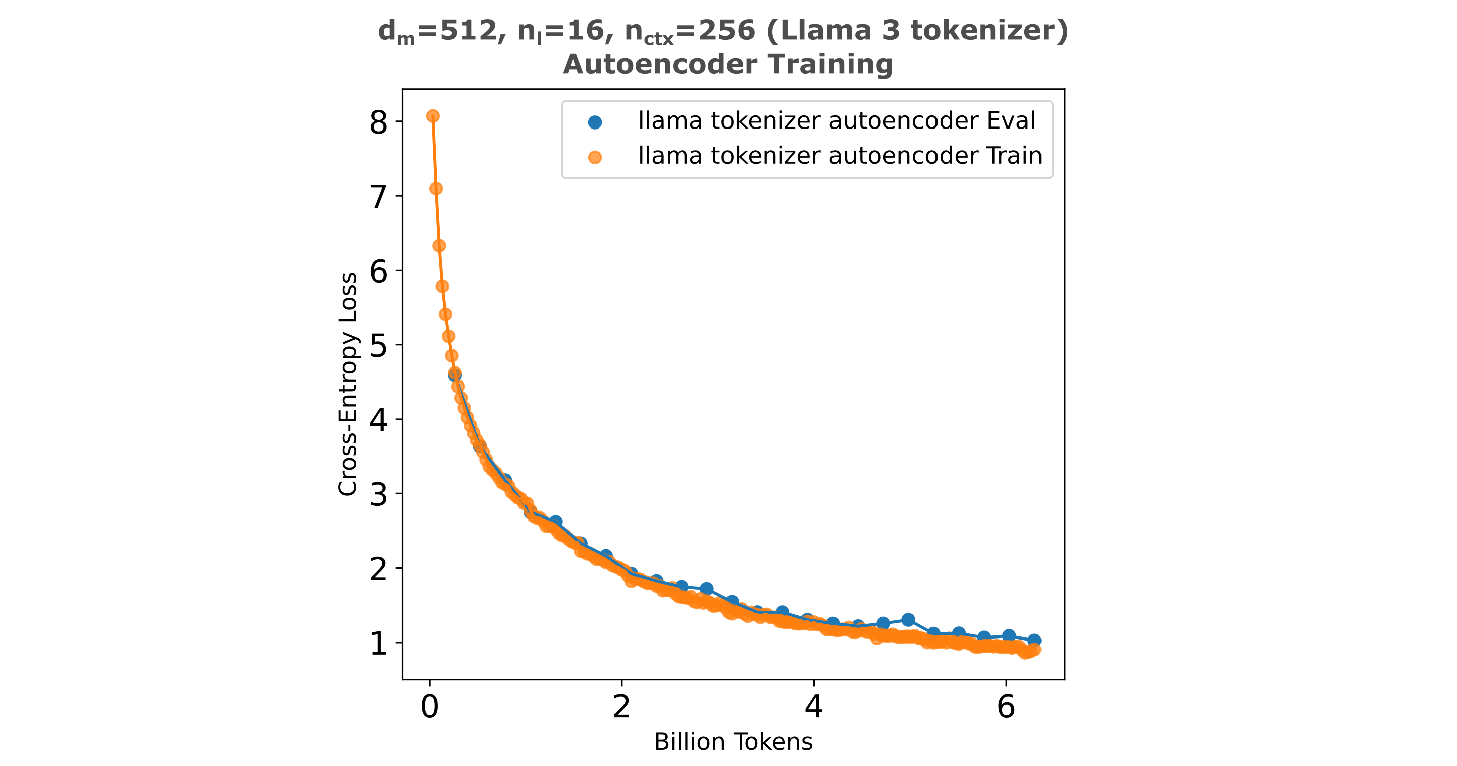
We then freeze the autoencoder’s encoder and feed the embeddings from this model to our pretrained Llama 3.2 (1b) memory model decoder and train on the same copy task as above. In the figure below, we provide a comparison to the trainable memory and no-memory Llama memory model training curves.
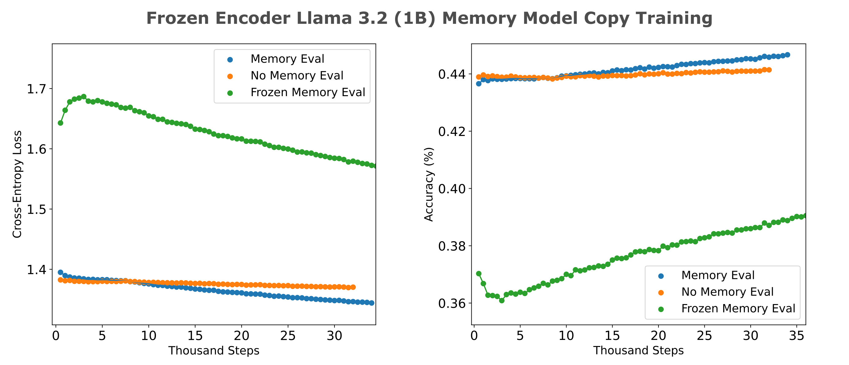
Given that copy training gives some ability for the decoder to access information in memory embeddings, it may be wondered whether this interferes with the modeling abilities of the pretrained decoder. We can test this by training the memory-enhanced Llama model, reformatting the decoder to match the original configurationa (ie a LlamaForCausalLM object), and benchmarking this model against the same model before copy memory model training. Early in training, we find that there is no decrease and actually a small increase in accuracy for most tasks.
Llama 3.2 (1B)
| Tasks | Version | Filter | n-shot | Metric | Value | Stderr | ||
|---|---|---|---|---|---|---|---|---|
| arc_easy | 1 | none | 0 | acc | ↑ | 0.6633 | ± | 0.0097 |
| none | 0 | acc_norm | ↑ | 0.6170 | ± | 0.0100 | ||
| hellaswag | 1 | none | 0 | acc | ↑ | 0.4805 | ± | 0.0050 |
| none | 0 | acc_norm | ↑ | 0.6427 | ± | 0.0048 | ||
| lambada_openai | 1 | none | 0 | acc | ↑ | 0.6222 | ± | 0.0068 |
| none | 0 | perplexity | ↓ | 5.4344 | ± | 0.1288 | ||
| mmlu | 2 | none | acc | ↑ | 0.3775 | ± | 0.0040 | |
| - humanities | 2 | none | acc | ↑ | 0.3515 | ± | 0.0069 | |
| - other | 2 | none | acc | ↑ | 0.4303 | ± | 0.0088 | |
| - social sciences | 2 | none | acc | ↑ | 0.4030 | ± | 0.0087 | |
| - stem | 2 | none | acc | ↑ | 0.3394 | ± | 0.0083 |
Llama 3.2 (1B), trained for memory copy, 2k training steps
| Tasks | Version | Filter | n-shot | Metric | Value | Stderr | ||
|---|---|---|---|---|---|---|---|---|
| arc_easy | 1 | none | 0 | acc | ↑ | 0.6629 | ± | 0.0097 |
| none | 0 | acc_norm | ↑ | 0.6174 | ± | 0.0100 | ||
| hellaswag | 1 | none | 0 | acc | ↑ | 0.4816 | ± | 0.0050 |
| none | 0 | acc_norm | ↑ | 0.6420 | ± | 0.0048 | ||
| lambada_openai | 1 | none | 0 | acc | ↑ | 0.6305 | ± | 0.0067 |
| none | 0 | perplexity | ↓ | 5.4167 | ± | 0.1283 | ||
| mmlu | 2 | none | acc | ↑ | 0.3858 | ± | 0.0040 | |
| - humanities | 2 | none | acc | ↑ | 0.3558 | ± | 0.0069 | |
| - other | 2 | none | acc | ↑ | 0.4419 | ± | 0.0088 | |
| - social sciences | 2 | none | acc | ↑ | 0.4176 | ± | 0.0088 | |
| - stem | 2 | none | acc | ↑ | 0.3444 | ± | 0.0083 |
But if we continue training, we find that there is indeed a degradation in benchmark accuracy as shown below:
Llama 3.2 (1B), trained for memory copy, 34k training steps
| Tasks | Version | Filter | n-shot | Metric | Value | Stderr | ||
|---|---|---|---|---|---|---|---|---|
| arc_easy | 1 | none | 0 | acc | ↑ | 0.6646 | ± | 0.0097 |
| none | 0 | acc_norm | ↑ | 0.5976 | ± | 0.0101 | ||
| hellaswag | 1 | none | 0 | acc | ↑ | 0.4638 | ± | 0.0050 |
| none | 0 | acc_norm | ↑ | 0.6159 | ± | 0.0049 | ||
| lambada_openai | 1 | none | 0 | acc | ↑ | 0.5960 | ± | 0.0068 |
| none | 0 | perplexity | ↓ | 6.4017 | ± | 0.1668 | ||
| mmlu | 2 | none | acc | ↑ | 0.2872 | ± | 0.0038 | |
| - humanities | 2 | none | acc | ↑ | 0.2837 | ± | 0.0066 | |
| - other | 2 | none | acc | ↑ | 0.3238 | ± | 0.0083 | |
| - social sciences | 2 | none | acc | ↑ | 0.2912 | ± | 0.0082 | |
| - stem | 2 | none | acc | ↑ | 0.2525 | ± | 0.0077 |
It is curious that the decrease in benchmark performance is particularly evident for MMLU (with a ~10% accuracy decrease) whereas there is little to no decrease for Arc-easy or Hellaswag. Arc and MMLU are both question-answering benchmarks, so it is unlikely that the MMLU degradation is strictly the result of training on a datsaet that is not specifically geared towards answering questions.
Autoencoders and memory models do not learn trivial encodings
Thus far we have seen curiously diverging training efficiencies with architectural changes for the case where the encoder’s embedding is as large or larger than the context window, versus the case where an encoder’s embedding is significantly smaller than the context window. For example, consider the widely different effect of using more mixer heads or a $k>1$ convolution for large embeddings (where this leads to much more efficient training) compared to small embeddings (where it leads to a decrease in training efficiency). Another example is the sharp drop in efficiency in both autoencoders and memory models as one decreases the encoder embedding size past the $n_{ctx}$ boundary.
Why would this occur? One hypothesis is that large-embedding models simply form trivial autoencodings that are easy to train and that this is assisted by the architectural modifications we have explored above, whereas it is impossible for small-embedding models to form trivial autoencodings. What is signified by a ‘trivial’ autoencoding is one in which the information from input token indices are passed to the output (or at least decoder) such that nothing is actually learned about the actual data distribution (educational text or mathematical text in this case).
A good example of a trivial autoencoding is for the case where the model’s context window is equal to the embedding dimension, $n_{ctx} = d_m$, and the model learns to represent each single input token as in a single embedding element. On this page we typically use a tokenizer of size 8000 and embeddings encoded in 16 bits per parameter. Clearly each embedding element can encode a token fairly accurately (for all tokenizers up to size $2^{16}=65536$), so a powerful autoencoder might simply learn this encoding.
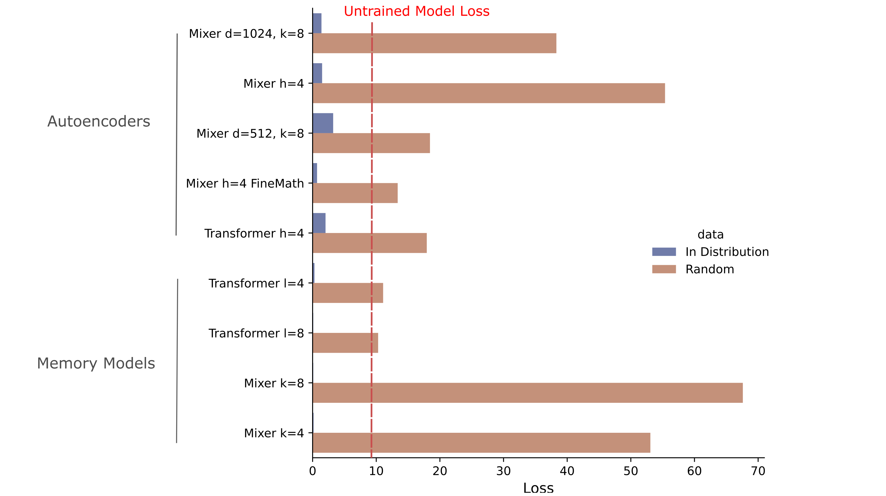
Testing for this one specific trivial encoding is not difficult, but one could imagine many other forms of equally distribution-free autoencoding such that it is difficult to directly test for all such encodings. Happily there is a somewhat direct way one can test for all trivial autoencodings as they are defined above: we can observe the loss (compression) for the model in question first on tokens that are drawn from a uniform random distribution and compare this to in-distribution loss. If nothing is learned about the actual data distribution, these values will be approximately equivalent.
Generating a uniform distribution on all possible tokens of a tokenizer is fairly straightforward: we can just check the size of an input and reassign the input as a tensor of random integers of the same shape.
input_ids = torch.randint(1, self.n_vocab, input_ids.shape)
For reference, we can decode these random inputs and confirm that they are indeed far outside the distribution of FineWeb-edu data, and the following shows that this is indeed the case.
adequate mot smart receive ruralgment wonvis requestusaloney |lessictues Pl legislationager guarduresiverse.comulin minutesí excessive ign-G blue pictures Environment kit hoursCE task enhanceuff oral Cast<|reserved_special_token_147|> individual.Cil Glick examined changing awayolesplace wid sector twenty du tox covered White<|reserved_special_token_13|> famouses influen.e
Does loss on these random tokens mirror loss on in-distriution data for large-embedding models, either autoencoders or memory models? The answer for both is no: across all models tested, the loss for these random strings is much larger than the in-disribution loss and indeed exceeds the untrained model loss (which is typically around 9.5). This is strong evidence against these models forming a trivial autoencoding as defined above.
Why does the untrained model have a loss of around 9.5? Untrained models (with either uniform or Kaiming normal weight initialization) typically exhibit activations that approximate Gaussian distributions, which is observed for vision models as well as for language models. As we are sampling tokens $n$ from a uniform distribution, we can compute the average cross-entropy loss between a normal distribution $\mathcal{N}$ over the tokenizer size (here $\vert t \vert = 8000$) and all possible token indices,
\[\frac{1}{n} \sum_n \Bbb L \left( \mathcal{N}((|t|, 0, 1), n \right) = 9.501\]Thus the loss we observe for our untrained model is nearly equivalent to the loss obtained if we assume that the activations of the output layer are approximately normal.
We can also observe the generalization of a given model by comparing the loss achieved on in-distribution versus marginally out-of-distribution data. We use FineMath as our marginally out-of-distribution dataset for models trained on the FineWeb, and FineWeb for models trained on FineMath. We have already observed good generalization for in-distribution data for most models on this page (there is <5% duplication between train and eval datasets for either FineWeb or FineMath but very little difference in train loss versus test loss).
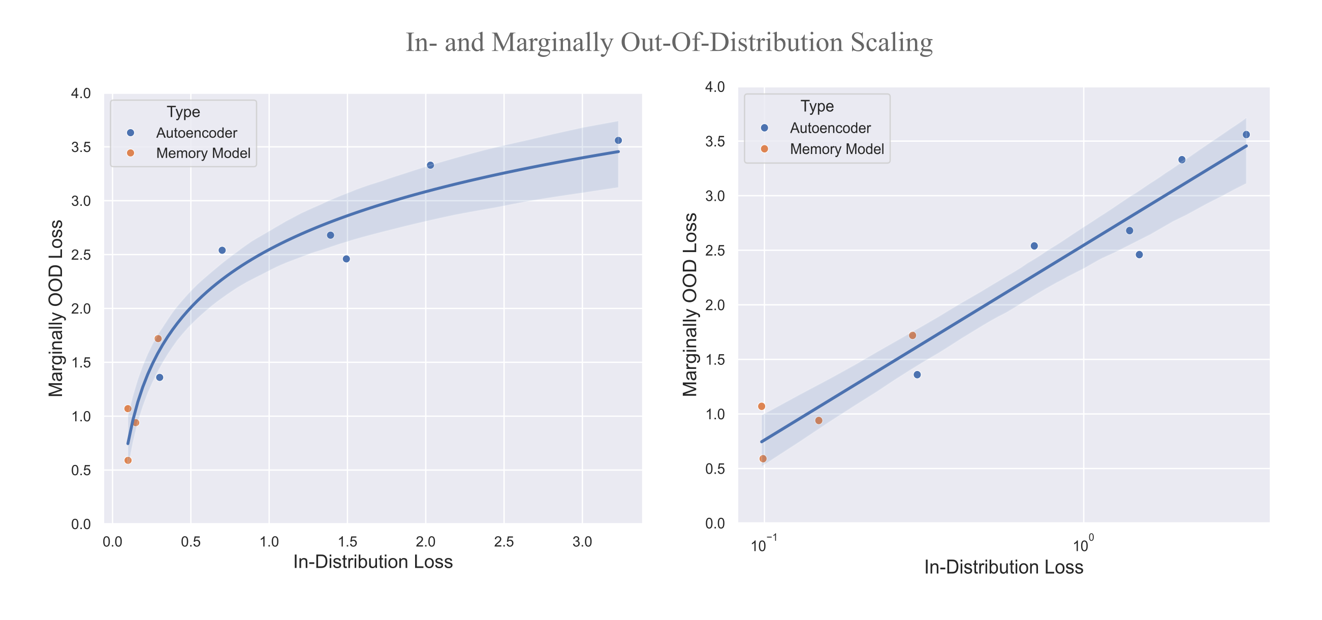
These results tell us that near-distribution generalization scales in a very similar manner between autoencoders and memory models. Curiously, however, masked mixer-based models of both types tend to be somewhat better generalizers than transformer models, as shown in the following figure.
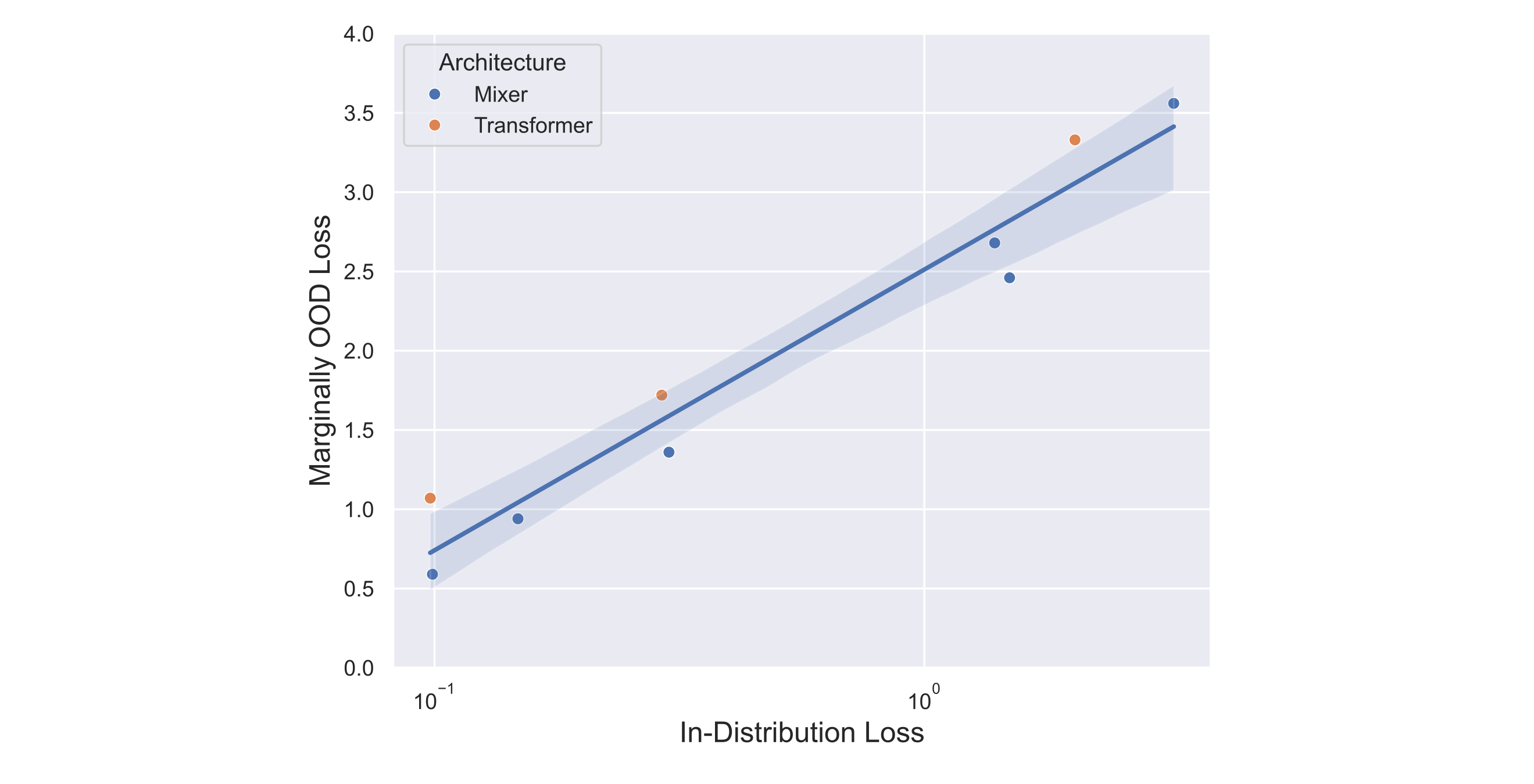
Thus neither memory models nor one-pass autoencoders learn trivial encodings, regardless of whether masked mixer or transformer architectures are used. It is natural to wonder next whether these models are even capable to learning a trivial encoding at all. As we observe nearly similar generalization properties for mixers and transformers, we may be free to pick either architecture and test the ability of a model that otherwise learns non-trivial autoencodings to learn a trivial autoencoding by simply training on uniform random tokens used earlier for evaluation.
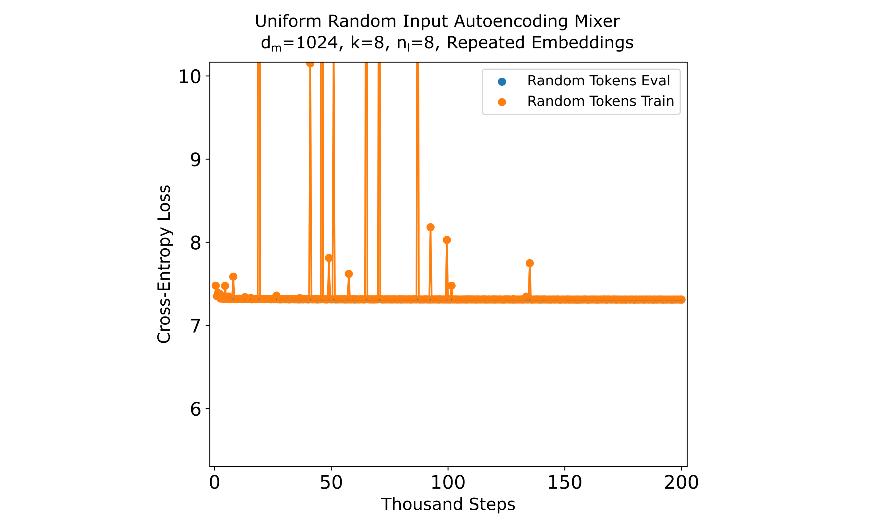
We employ an efficiently-trainable autoencoder architecture ($n_{ctx}=512, d_m=1024, k=8$ with $n_l=8$ for both encoder and decoder and repeated embeddings in the decoder) that is capable of reaching ~0.6 CEL on FineMath or ~1.5 on FineWeb after training on 13 billion tokens. We use bf16/fp32 mixed precision training after encountering numerical instabilities when using fp16/fp32 mixed precision training using this dataset.
As shown in the following figure, this autoencoder experiences virtually no loss minimization and thus does not learn a trivial autoencoding on these random tokens.
How much information do embeddings contain?
We have seen that one can train autoencoders to compress information from many tokens into the embedding of one, and that this compression is non-trivial and reflects the distribution of the training data. This means that the embeddings of these autoencoders (the encoder’s embedding passed to the decoder) is capable of near-lossless 512:1 compression with respect to token embeddings.
It may be wondered whether this is at all remarkable: after all, one can train a language model in many ways such that it is possible that many types of training will result in similar information compression characteristics. Does this compression result if we train models objectives that are more common in the field, such as causal modeling to predict next tokens or noise-contrastive estimation for retrieval?
To restate, this section will address the following question: how much information is contained in embeddings from models trained for different tasks? It is often assumed that large models trained with lots of compute will be best at most tasks, but is this true if the task requires much or all of the information in the input to be compressed into an embedding?
Our experimental design is as follows: we load the weights of the encoder model of whichever type we want, discard the word-token embedding and language modeling head (and decoder if relevant), freeze the blocks, and train a decoder (and word token embedding transformation) to minimize the autoencoding loss on the dataset that the encoder was trained on (here FineWeb 10BT). With one decoder architecture and fixed-compute encoders, we can get an idea of how much information is present in these embeddings if we can train the decoder to convergence, or at least sufficiently close to convergence. We train on the same context window used for encoder training ($n_{ctx}=512$) and the decoder is of size ($d_m=1024, n_l=8$). We repeat the embedding unless otherwise noted.
We first consider these questions for masked mixers. As a positive control, we can confirm that this approach is capable of recovering nearly all the information present in an autoencoder’s embedding (below left) when the decoder recieves an unrolled projection of the embedding. This shows that our decoder-only training approach is sufficient to recover most of the information present in the embedding.
In the following figure, we find that causal (next-token) training results in a small increase in informational content of a model’s embedding (here second-to-last token embedding as the last token is untrained) compared to an untrained model, and that an embedding (at the same position) from a noise contrastive encoding retrieval model has somewhat increased informational content relative to the causal model. This indicates that the retrieval training process increases information retention, as this model was first trained for causal modeling before InfoNCE-based retrieval training was applied.
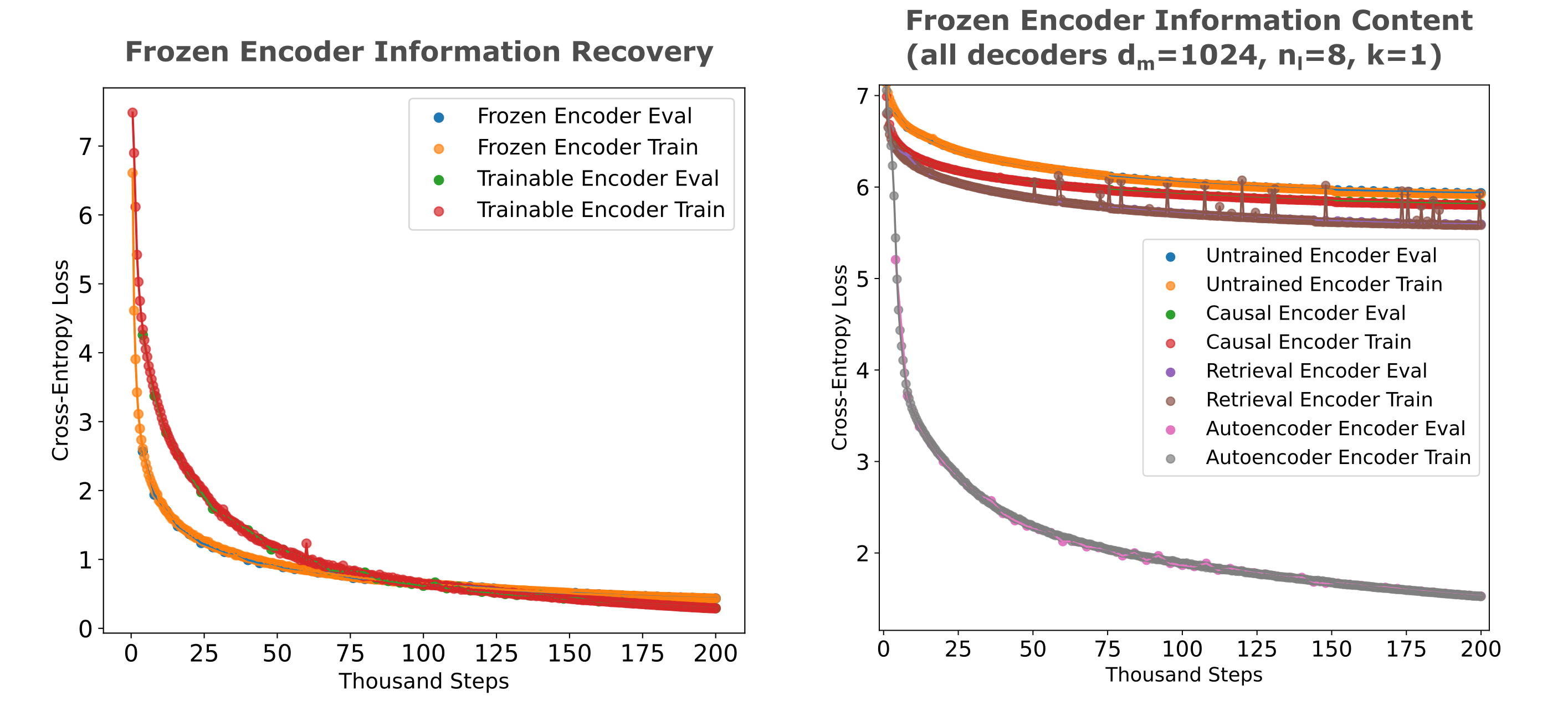
We see slightly less information recovery from a frozen transformer’s encoder compared to what was observed for mixers, and the same general small increase in information retention for causal models compared to untrained ones. Curiously there is actually a small decrease in embedding information for retrieval models relative to causal models, which may provide some basis for the finding that mixers are generally more efficient for retrieval.
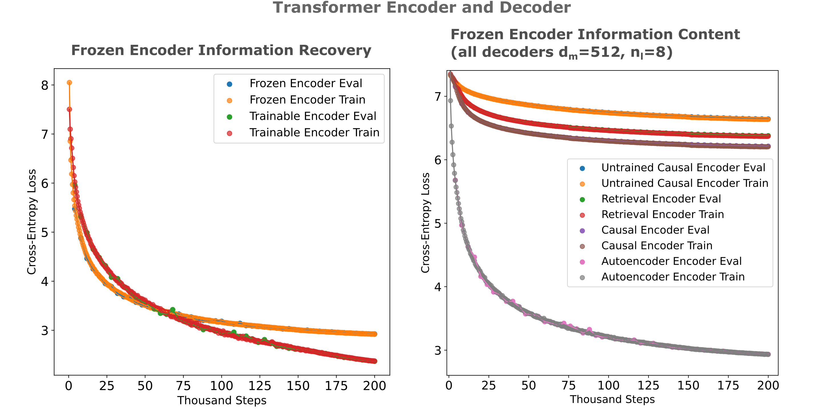
For both model architectures, retrieval and causal embeddings contain only a small fraction of the information compared to the autoencoder embedding. This is not a subtle difference, and it cannot be reasonable argued that extended training of the decoder would result in any other conclusion.
The natural question to ask is how much information these cross-entropy loss values represent. The answer depends on our definition of information: one could define information as a Hamming metric on the tokenized output and target (input) tokens, such that the information present in the embedding is a measure of the proportion of correct tokens predicted. We employ a modified version of the normalized Hamming metric introduced here, which to recap is defined as the proportion of tokens in non-pad indices (as defined by the target sequence $x$) where the target’s token does not match the model’s output $y$. More precisely, for sequences of input tokens $x$ and tokens generated by the target $y$ with tokenizer size $t_m$,
\[x = (x_1, x_2, ..., x_n), \; y = (y_1, y_2, ..., y_n) \in \{0,1,...,t_m\}^n\]we then find the cardinality (size) of the set of tokens at position $i$ where the target token index does not match the model output token index, ignoring padding tokens, and divide this number by the number of non-pad tokens $j$ and take the complement:
\[h(x, y) = 1 - \frac{1}{j} \mathrm{Card} \left( \{ x_i \neq y_i \} \right) : x_i \neq t_{pad}\]Alternatively, we can define information retention using the cross-entropy as the fraction of cross-entropy loss the model reaches over the loss of an ‘informationless’ model. In this definition we want to understand what the cross-entropy losses would be for a model with perfect information and a model with no information, and normalize our obtained losses by these values. A model with perfect information in its encoder will clearly obtain zero cross-entropy loss (assuming an arbitrarily powerful decoder). The distribution with the least Shannon information is the uniform ($\mathbf U$) distribution by definition, so we can compute the cross-entropy loss corresponding to an informationless model by simply assuming that the model exhibits a uniform distribution $\mathcal{U} \sim [0, 1)$ over token activations. As our tokenizer is of size $\vert t \vert =8000$, we compute the following for $n \to \infty$ tokens:
\[H(p_0, q) = \frac{1}{n} \sum_{n} \Bbb L \left( \mathcal{U}(|t|), t \right) = 9.03\]where $t$ is sampled from the input distribution, or equivalently any distribution given that the reference is uniform, such that we have a range of $\Bbb L \in [0, 9.03]$ for our tokenizer. We can therefore define the embedding information as the complement of the fraction of our cross-entropy loss
\[I_e = 1 - \frac{H(p, q)}{H(p_0, q)} = 1 - \frac{- \sum_x q(x) \log (p(x))}{- \sum_x q_0(x) \log (p(x))}\]which for our 8k-size tokenizer we have
\[I_e = 1 - \frac{H(p, q)}{9.03}\]Whereas for Llama 3.2 (1B) with a tokenizer of size 128256 we have $I_e = 1 - \frac{H(p, q)}{11.80}$, for BERT with a 30522 size tokenizer $I_e = 1 - \frac{H(p, q)}{10.37}$ and for Qwen 3 with a tokenizer of size 151688 we have $I_e = 1 - \frac{H(p, q)}{11.97}$
For mixers, we have the following:
| Encoder Model | Loss | Entropy proportion $I_e$ | Hamming $1-h(x, y)$ |
|---|---|---|---|
| Autoencoder (validation) encoder | 0.435 | 0.952 | 0.7696 |
| Autoencoder encoder | 1.528 | 0.831 | 0.5534 |
| Untrained | 5.937 | 0.343 | 0.0408 |
| Causal Trained | 5.815 | 0.356 | 0.0479 |
| Causal -> Retrieval Trained | 5.594 | 0.381 | 0.0476 |
| Autoencoder -> Retrieval Trained | 5.767 | 0.361 | 0.0447 |
and for transformers,
| Encoder Model | Loss | Entropy proportion $I_e$ | Hamming $1-h(x, y)$ |
|---|---|---|---|
| Autoencoder (validation) encoder | 2.924 | 0.676 | 0.3882 |
| Autoencoder encoder | 2.935 | 0.675 | 0.391 |
| Untrained | 6.643 | 0.264 | 0.0409 |
| Causal Trained | 6.214 | 0.311 | 0.0462 |
| Causal -> Retrieval Trained | 6.380 | 0.293 | 0.0438 |
By this metric, therefore, we observe that causal language and retrieval model training result in small increases in information retention, on the scale of 1-4%, compared to untrained models but that autoencoder training results in an order of magnitude larger information retention increase. We conclude that causal models trained here do not retain most input information (and indeed barely more than untrained models) and somewhat suprisingly neither do retrieval models, whereas autoencoders are capable of retaining most or nearly all input information, depending on the sequence length.
LLM Information Retention
The conclusion reached in the last section is notably different from that obtained in another study using similar techniques to measure informational content in large causal transformers by Morris and colleagues. There, those authors found that one can achieve at least somewhat accurate inversion of models using output logits of a next token predicted after a hidden prompt is fed to the model. We note that this is likely due to two notable differences: there, the authors were interested in regenerating prompts rather than entire text segments, and accordingly train decoders using a context window of 64 tokens rather than the 512 tokens used here. Most models in that work are furthermore much larger than those considered here, and the dataset considered is much more restricted (sytem prompts rather than arbitrary text) and when that inversion process was performed using general text, accuracy was much reduced. Here and Elsewhere it was observed that information retention in an embedding is highly dependent on context window size with smaller contexts being much easier to retain information from. In this light, the finding that causal models struggle to retain most information of arbitrary text with much larger context window is perhaps unsurprising.
These observations yield the following question: given that small and relatively low-resourced causal and retrieval models are not observed to retain much input information, how much information do larger language models (particularly those trained with much more compute) retain? We effectively seek to determine whether our results are particular to relatively small models trained with few (10s of billions or) tokens or whether they are general to the training objectives of language training.
Firstly we consider a widely used embedding model: BERT, which is around twice the size (in terms of parameter count) as the causal transformer models introduced above and trained with around 10x the compute (using modern distributed training software, around 1k V100-hours compared to the 100 V100 hours used for our transformer models). This model was trained using the masked language objective, and has been used extensively for retrieval. Much work has been performed to understand what BERT embeddings can do, and the conclusion is that they can do quite a lot: one can use them for next token prediction, sentiment analysis, summarization, retrieval, and much more.
Our experimental procedure is as follows: we seek to understand the amount of input information present in a model by initializing and freezing it and training a decoder to regenerate input sequences of various lengths from the last hidden layer’s last embedding of the frozen LLM. Some experimentation suggests that the decoders train more efficiently when the entire LLM is frozen including the word token embedding, which is the opposite of what was observed for the transformer models noted above which have a slight increase in decoder training efficiency when the WTE transformation was unfrozen and trainable. We also find that decoders need not be nearly as large as encoders: using a $d_m=1024, n_l=16, h=4$ Llama-style decoder rather than the BERT-large $d_m=1024, n_l=24, h=16$ actually results in increased training efficiency, and reducing this further to a $d_m=512, n_l=16, h=4$ decoder leads to no performance decrease. Aside from these denoted differences, however, the architecture of the full encoder-decoder with unrolled encoder embeddings is identical to that detailed previously.
In addition to BERT-large we also investigate the causal language modeling-trained Llama 3.2 (1B), which is around 6x the size of our models and was trained on many orders of magnitude more data and compute. The results of inverting these models on FineWeb inputs are denoted in the table below, where at each context length the cross-entropy loss and input token recovery accuracy (%) are given.
| Model | n_{ctx}=16 | 64 | 256 | 512 |
|---|---|---|---|---|
| BERT large | 2.91 (40.2%) | 5.38 (11.6 %) | 6.16 (6.6 %) | 6.47 (5.96 %) |
| Llama 3.1 (1B) | 3.95 (34.8 %) | 6.02 (11.2 %) | 6.68 (6.0 %) | 6.86 (5.3 %) |
| BERT (FineMath) | 1.13 (72.3 %) | 3.72 (26.8 \%) | 4.89 (12.6 \%) | 5.28 (9.6 %) |
It is clear that there is a substantial decrease in information retention as context length increases, but even for the small 16-token context we observe that only a minority of tokens may be accurately recovered from the last hidden layer with our compute applied. We observe a slight decrease in information retention for the larger and (much) more compute-trained Llama 3.1 than BERT, although both models exhibit near-identical accuracy for $n_{ctx}=512$ token context windows as our smaller causal transformers as shown in the last section.
As accurate small-context LLM information recovery using similar architectures (specifically via unrolled embeddings with endoer-decoder sequence-to-sequence models acting as the decoder) has been observed by Morris and colleagues for inputs restricted to system prompts, we investigated whether or not restriction of the corpus over which we train our decoder would result in higher information retention fidelity. We test this by training on a mathematical subset of the FineWeb dataset (FineMath-4+), and find that this is indeed the case: small-context token recovery nearly doubles for BERT relative to the more diverse FineWeb, suggesting that indeed a restriction of input diversity results in easier information recovery, presumably due to higher relative compression ability. The increased accuracy for restricted versus unrestricted corpora is evident at larger context windows as well, but it should be noted that there is again a substantial decrease in input recovery as the context length increases.
In conclusion, larger models trained with (vastly) more data and compute does not yield more accurate input representations, either for masked or causal language models. This implies that it is not compute or data scaling but the tasks themselves that determine information retention: causal and masked language models do not retain very much input information simply because these tasks do not require much input information to complete accurately. This is presumably because all input tokens are given to these models for each token prediction step, so the models are trained to filter rather than store the informatino present in the inputs.
Causal Memory Models Memories don’t have much Information
The trainable memory models introduced earlier on this page have a severe disadvan tage to full-context models: their memories, once made, are fixed. This is a significant problem because many tasks language models are applied to today require near-arbitrary lookup of previous tokens (‘Can you tell me what day Bob was in town as mentioned in the document…’), but this lookup is essentially unpredictable without prior knowledge. Due to the inherent degrees of freedom of a user’s input, lookup is fundamentally unpredictable in the sense that the model has no way of knowing what the user will ask for in the general case.
This is not a problem for full-context decoders because they are exposed to perfect input information, as all tokens are visible to the model at all times. This means that it does not matter (for autoregressive decoding purposes) that these models have rather poor input representation: as long as each single token predicted requires information from only a subset of previous tokens, accurate input representation is superflouous and probably detrimental to a causal decoder. A brief reflection may convince one that it is indeed the case that nearly all predicted tokens require knowledge of only one or a few previous tokens for most tasks (certainly for the question above).
The issue here is that memory model decoders are not exposed to perfect input information in the general case, only the information that the encoder was trained to retain during the causal language model training process. This means that unless the encoder happened to capture the necessary information for all future queries on the input, the decoder cannot answer all queries accurately. This observation motivates the following question: how much information do memory model encodings (trained for next token prediction) actually contain? The hypothesis is that because causal language modeling typically does not require much information from long-past tokens, memory model encodings will not contain much input information.
We test this as follows: a trained memory model is initialized and the decoder discareded, and the encoder is frozen and added to an autoencoder decoder such that the last token from the encoder is unrolled and fed to the decoder, and the decoder is then trained to regenerate in-distribution input sequences. Specifically we seek to mirror the ratio of $n_{ctx}:d_m$ that we have explored above, which for masked mixers is $1:2$ and for transformers $1:1$. For masked mixers we use a trained memory models with a $n_{ctx}=256, d_m=512$ encoder and for the transformer a $n_{ctx}=512, d_m=256$ encoder.
When this experiment is done, we find that our hypothesis is indeed supported: masked mixer-based memory encoders exhibit nearly identical CELs to causal models with the same $d_m:n_{ctx}$ ratio, meaning that we can expect to recover around 5% of all tokens in the input sequence. For a transformer-based memory encoder with a smaller $d_m:n_{ctx}$ ratio than for causal models we find that the information retention is also correspondingly somewhat lower (left, below).
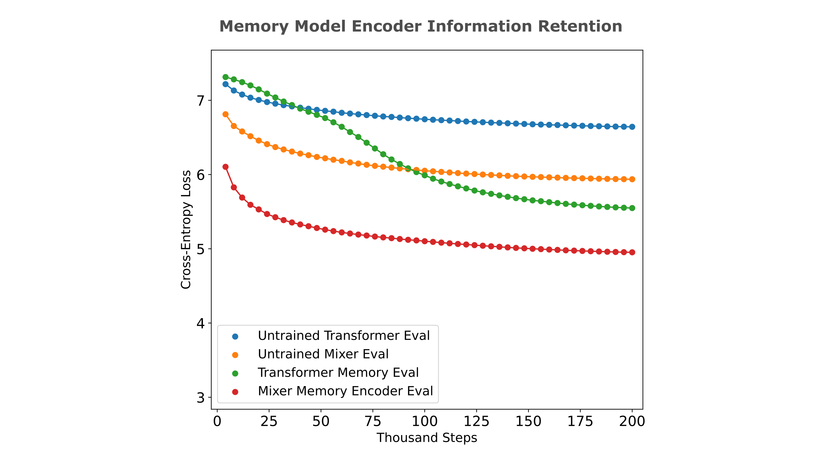
We can also perform a somewhat more direct experiment to address the question of how much information memory model (trained for next token prediction) encodings contain: we copy the first half of each FineWeb input to the second half, load and freeze the encoder from a trained memory transformer, and mask the second half the the inputs before each forward pass (the labels, ie the target values, remain exposed to the model). This is the ‘blank copy’ experimental procedure outlined previously, and this measures the amount of information that the encoder’s embeddings are capable of relaying to the decoder as the decoder is not exposed to any other source. We can compare blank copy training efficiency using (frozen) causal, non-memory models, causal memory model encoders, and compressive autoencoders in order to understand the accessible informational content in each encoder.
In the figure below (right), we see the results of doing so: autoencoder encoders are far more information-rich than causal or memory model encoders, the latter of which contain only a small fraction more information than the causal model.

Thus we find evidence for the idea that memory model encoders do not actually store much information from their inputs when these models are trained to predict next tokens, presumably because the task of prediction of most next tokens in a general corpus does not actually require much information from previous tokens.
Oracle memories are compressed even if they don’t need to be
We can also use this method to determine the informational content of the embedding-augmented ‘oracle’ memory models introduced in an earlier section on this page. Recall that these models combine an encoder with a causal language modeling decoder, and for large-dimensional (ie $d_m \geq n_{ctx}$) transformers and mixers with some mild architectural constraints these models approach 0 loss with limited training budgets. This begs the question: how much information is contained in the embedding generated by the encoder? One estimate is as follows: given that the decoder-only models achieve a CEL of ~2.6 on this dataset, so we achieve a bits-per-byte compression of
\[\mathtt{BPB} = (L_t/L_b) \Bbb L / \ln(2) = (1/3.92) * 2.60 / \ln(2) \approx 0.957\]with the decoder alone. With the encoder, we have a compression (disregarding the encoder) of
\[\mathtt{BPB} = (L_t/L_b) \Bbb L / \ln(2) = (1/3.92) * 0.1 / \ln(2) \approx 0.036\]meaning that the encoder is responsible for approximately 0.921 bits per byte, which is not very remarkable given that the encoder’s amortized memory for these large models results is 8 bits per byte extra. This is not nearly enough to accurately compress the 512 token context window, however, as shown below:
If we compute the information metrics used previously
| Encoder Model | Loss | Entropy proportion $I_e$ | Hamming $1-h(x, y)$ |
|---|---|---|---|
| Mixer memory (repeat) | 4.953 | 0.451 | 0.1390 |
| Mixer memory (unrolled) | 4.980 | 0.449 | 0.1589 |
| Transformer memory (unrolled) | 5.549 | 0.385 | 0.0842 |
Thus the large-dimensional oracle memory embeddings contain more input information than causal model embeddings and untrained models, but still only exhibit retention of a fraction of the total information in the input. Recall previous results showing that that this relatively low-information embedding results in better next token prediction than a frozen high-information autoencoder embedding when paired with a causal decoder. As the decoder is fed all previous tokens at each forward pass, this suggests that a small amount of input information is necessary to provide next token information when paried with this previous token information.
How much information does this memory model encoder embedding contain compared to its capacity in terms of bits per bytes? After training our decoder, we have a BPB compression of
\[\mathtt{BPB} = (L_t/L_b) \Bbb L / \ln(2) = (1/3.92) * 4.93 / \ln(2) \approx 1.81\]whereas the amortized bits per input byte of the embedding ($d_m=1024, n_{ctx}=512$) assuming no compression is
\[\mathtt{BPB} = \frac{n_p * b_p}{n_{ctx} * (L_b / L_t)} = \frac{1024 * 8}{512 * 3.92} \approx 4.08\]Thus the encoder has learned to compress the input by a factor of 1.81:4.08, even though it would not have to in the sense that an uncompressed embedding contains 4.08 bits per input byte of information which would be sufficient for allowing the decoder to achieve zero loss.
Equivalently we have an input of 512 tokens each containing 3.92 bytes, we have an input of 2007 bytes and thus our encoder contains around 2007 bytes * 1.81 bits/byte = 3633 bits of information per context window. This is much smaller than the (uncompressed) 1024 parameters * 8 bits/parameter = 8096 bits present in the encoder’s embedding, assuming 8 bits per parameter quantization.