Transformer and Mixer Features

Vision Transformer Feature Visualization

Convolutional models consist of layer of convolutional ‘filters’, also known as feature maps, that tend to learn to recognize specific patterns in the input (for a detailed look at this phenomenon, see this page). These filters are linearly independent from one another at each layer, which makes it perhaps unsurprising that they would select for different possible input characteristics.

At first glance, it would appear that transformers do not contain such easily separated components because although each input is separated into a number of patches that are encoded in a linearly separable manner, the attention transformations act to mix this information, moving relevant information from one token (in this case a patch) to another. For an interesting look at this in the context of attention-only transformers applied to natural language, see this work by Elhage and colleagues.

But we can investigate this assumption by performing a feature visualization procedure similar to that undertaken for convolutional image models on this page. In brief, we seek to understand how each component of a model responds to the input by finding the input which maximizes the activation of that component, subject to certain constraints on that input in order to make it similar to a natural image.

More precisely, we want to find an input $a’$ such that the activation of our chosen model component $z^l$ is maximized, given the model configuration $\theta$ and input $a$, denoted by $z^l(a, \theta)$

\[a' = \underset{a}{\mathrm{arg \; max}} \; z^l(a, \theta)\]

Finding the exact value of $a’$ can be very difficult for non-convex functions like hidden layer outputs, so instead we perform gradient descent on an initially random input $a_0$ such that after many steps we have an input $a_g$ that approximates $a’$ in that the activation(s) of component $z_l$ is maximized subject to certain constraints. The gradient here is the tensor of partial derivatives of the $L_1$ metric between a tensor with all values equal to some large constant $C$ and the tensor activation of the element $z^l$

\[g = \nabla_a (C - z^l_f(a, \theta))\]

At each step of the gradient descent procedure, the input $a_k$ is updated to $a_{k+1}$ as follows

\[a_{k+1} = \mathscr J \left( \mathcal N_x(a_k - \epsilon * g_k) \right)\]

where $\mathcal N$ signifies Gaussian blurring (to reduce high-frequency input features) and $\mathscr J$ is random positional jitter, which is explained in more detail here.

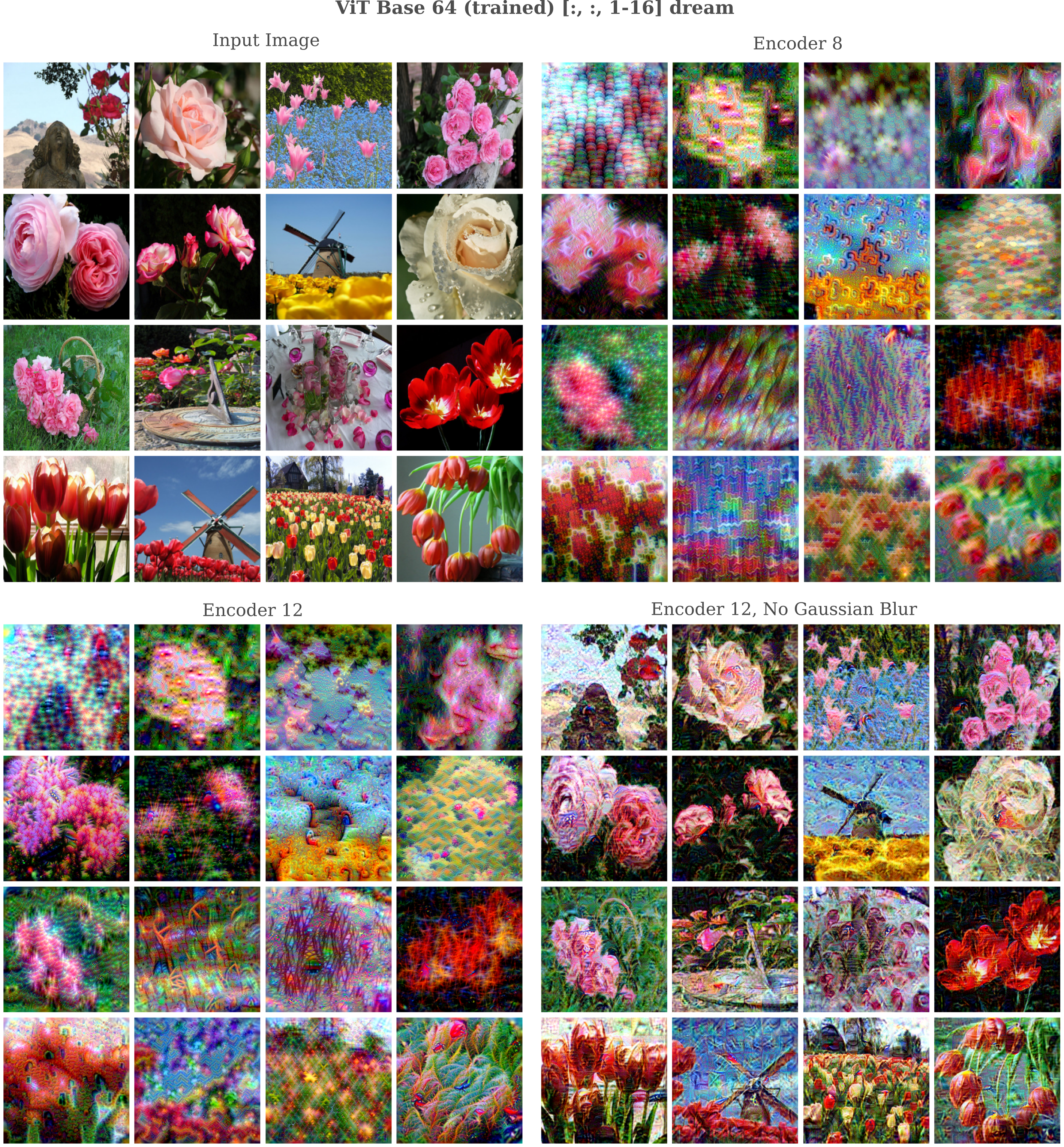
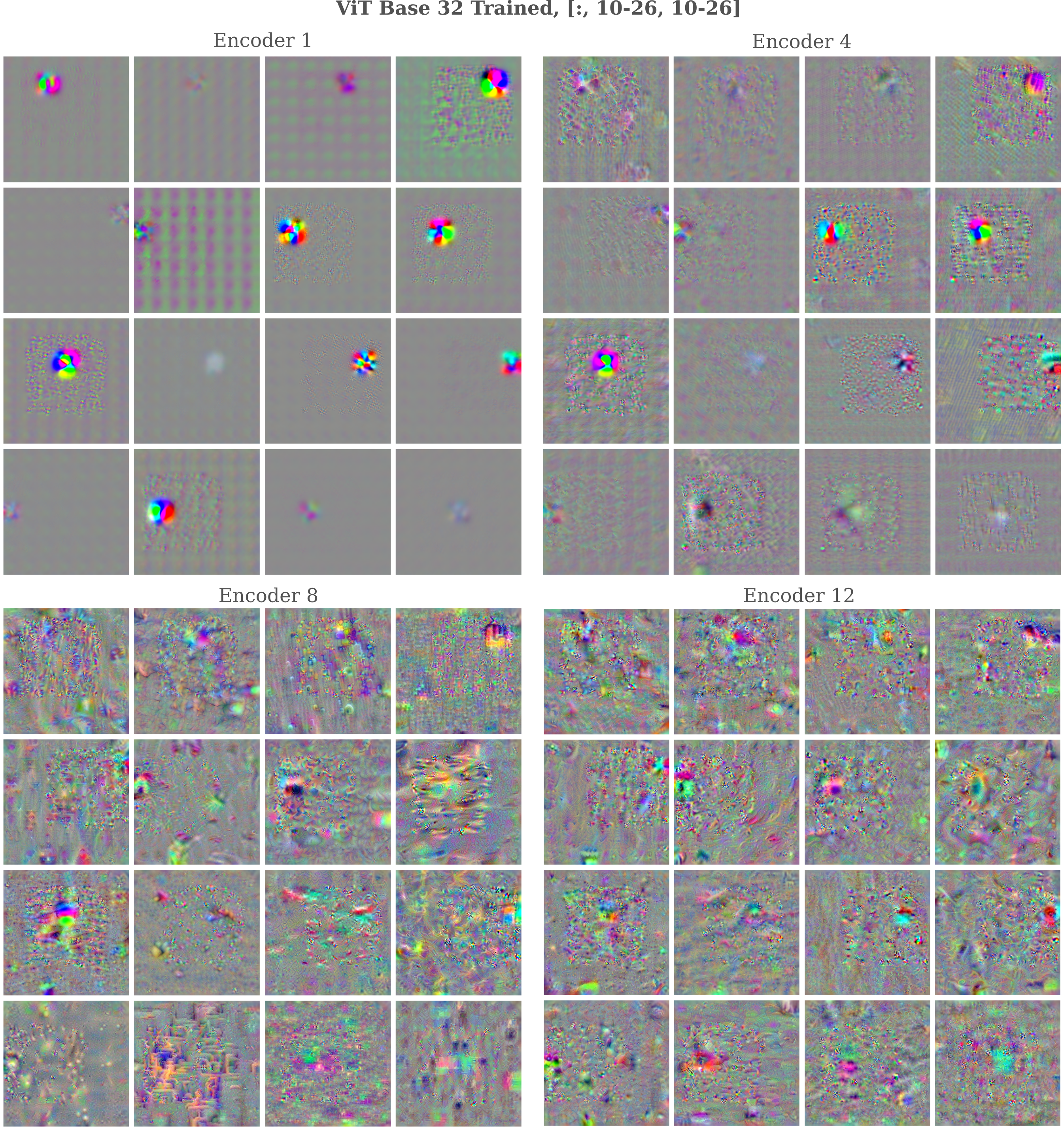
For clarity, the following figure shows the shape of the tensors we will reference for this page. We will focus on the generated inputs that result from maximizing the activation of one or more neurons from the output layer of the MLP layers in various components.

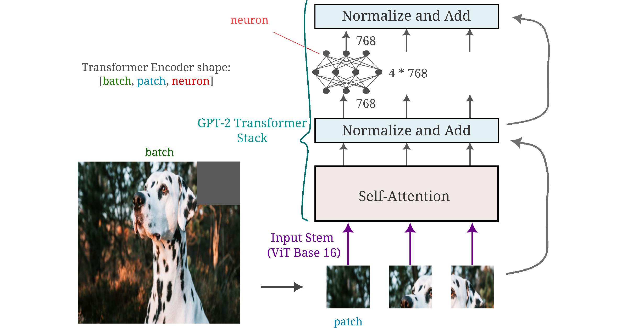
It is important to note that the transformer’s MLP is identically applied across all patches of the input, meaning that it has the same weights and biases no matter where in the image it is applied to. This is similar to a convolutional operation in which one kernal is scanned across an entire image, except that for the vision transformer the feature information is stored in individual MLP neurons, whereas for convolutional models typically there are multiple neurons (3x3 and 5x5 are common convolutional filter sizes) required per feature.

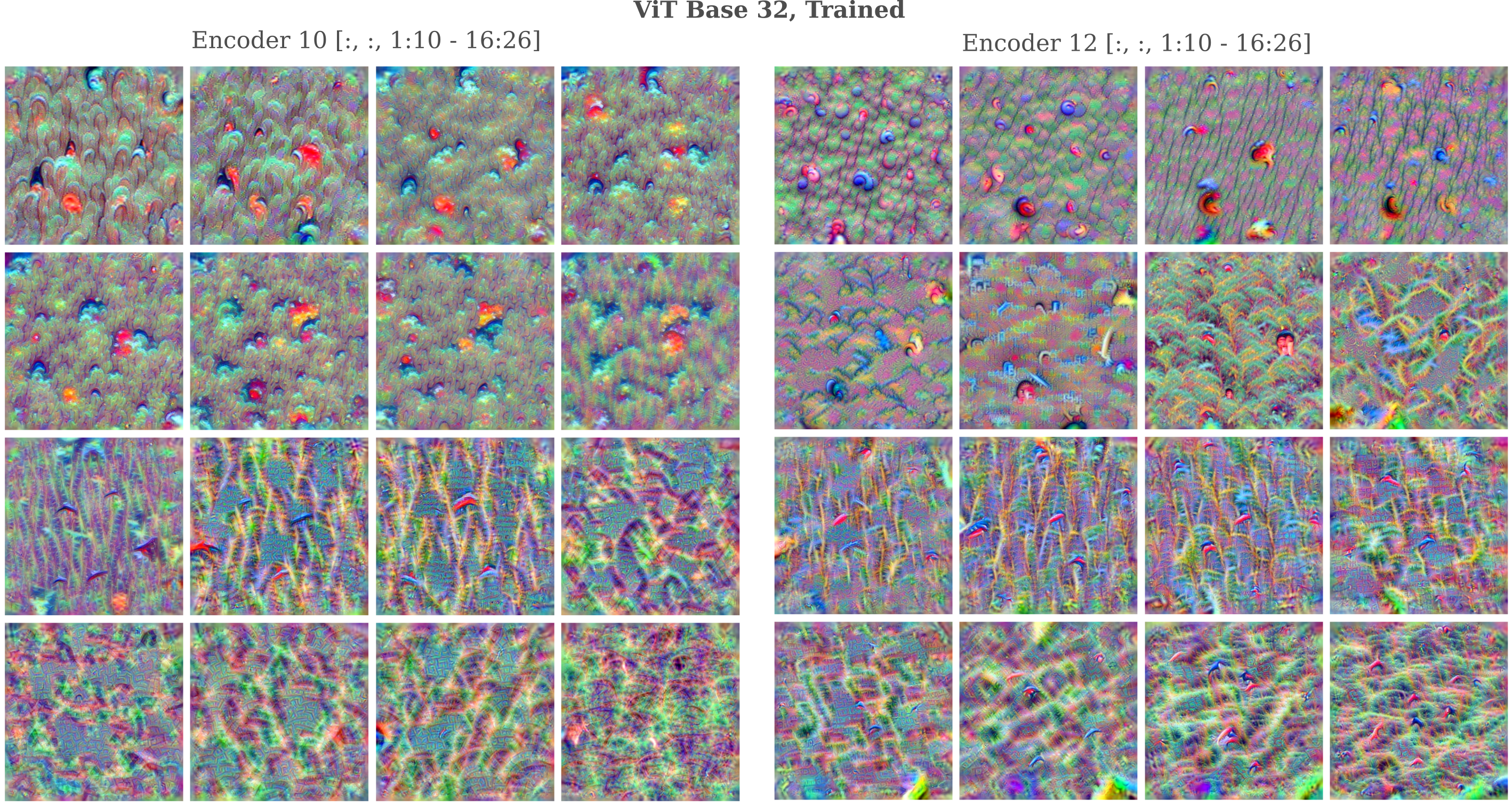
For Vision Transformer (ViT) base with 32x32 pixel patches (with 88M parameters total) we have

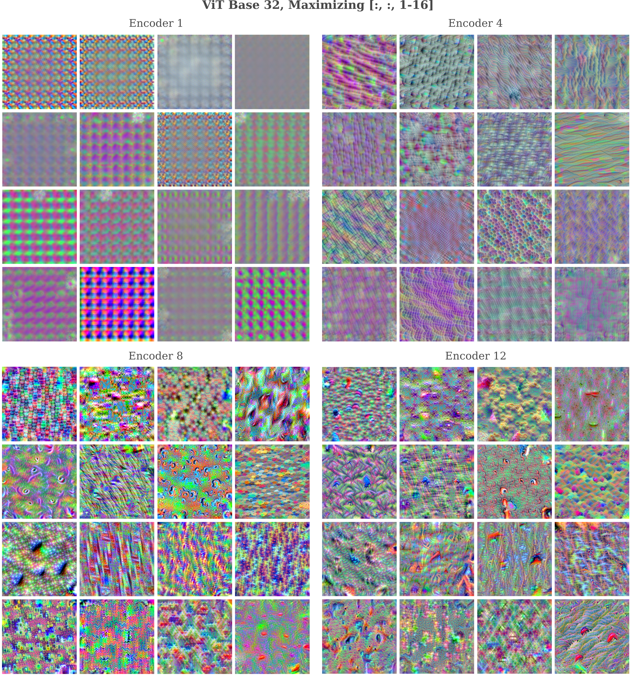
Maximizing the activation of a subset of neurons in all patches yields the following feature maps:

For single neurons in individual patches we have

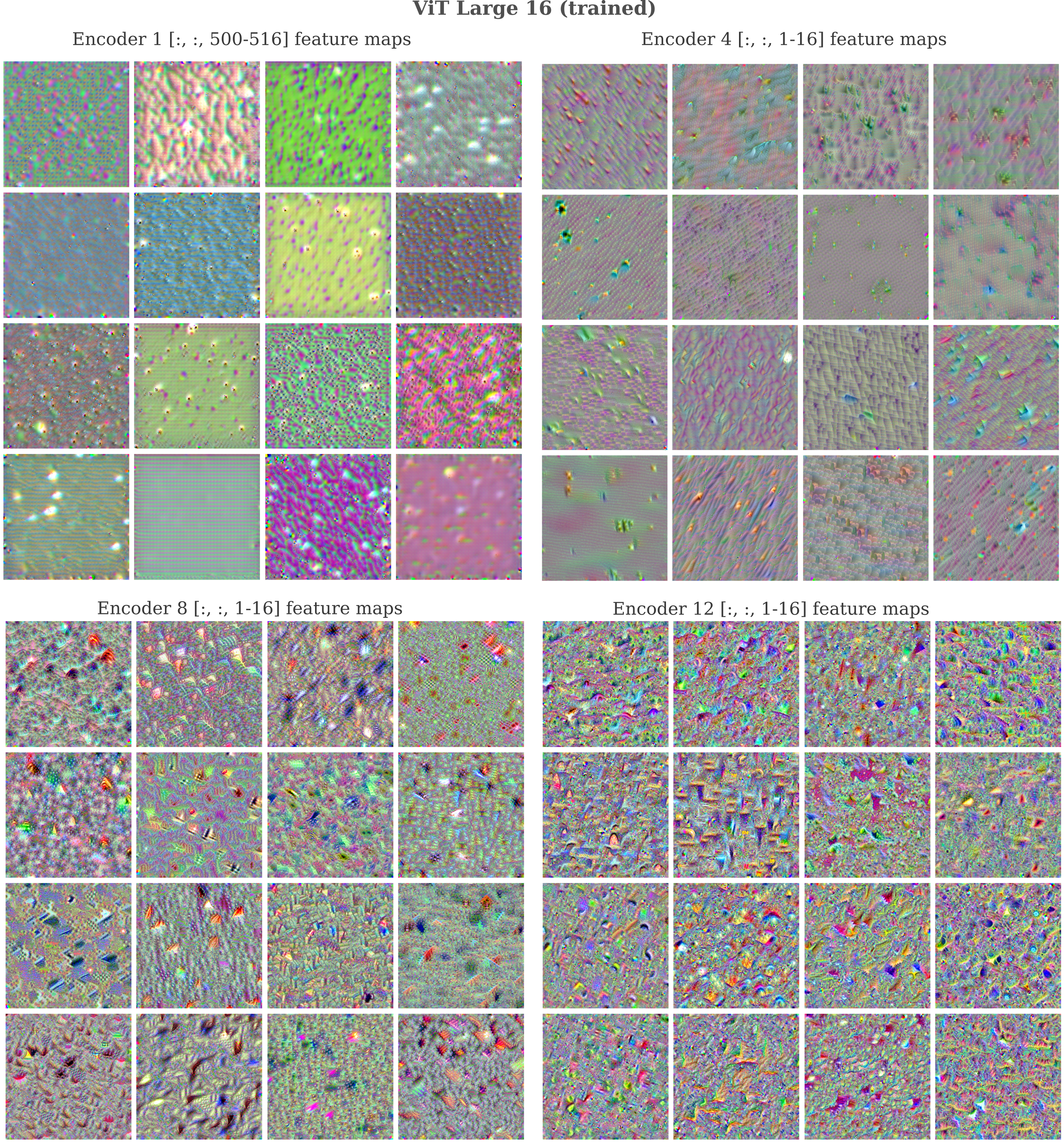
Similarly when we observe features of ViT Large 16 (which contains ~300M parameters in this configuration) which underwent weakly supervised pretraining before ImageNet training, we have

MLP Mixer Feature Map

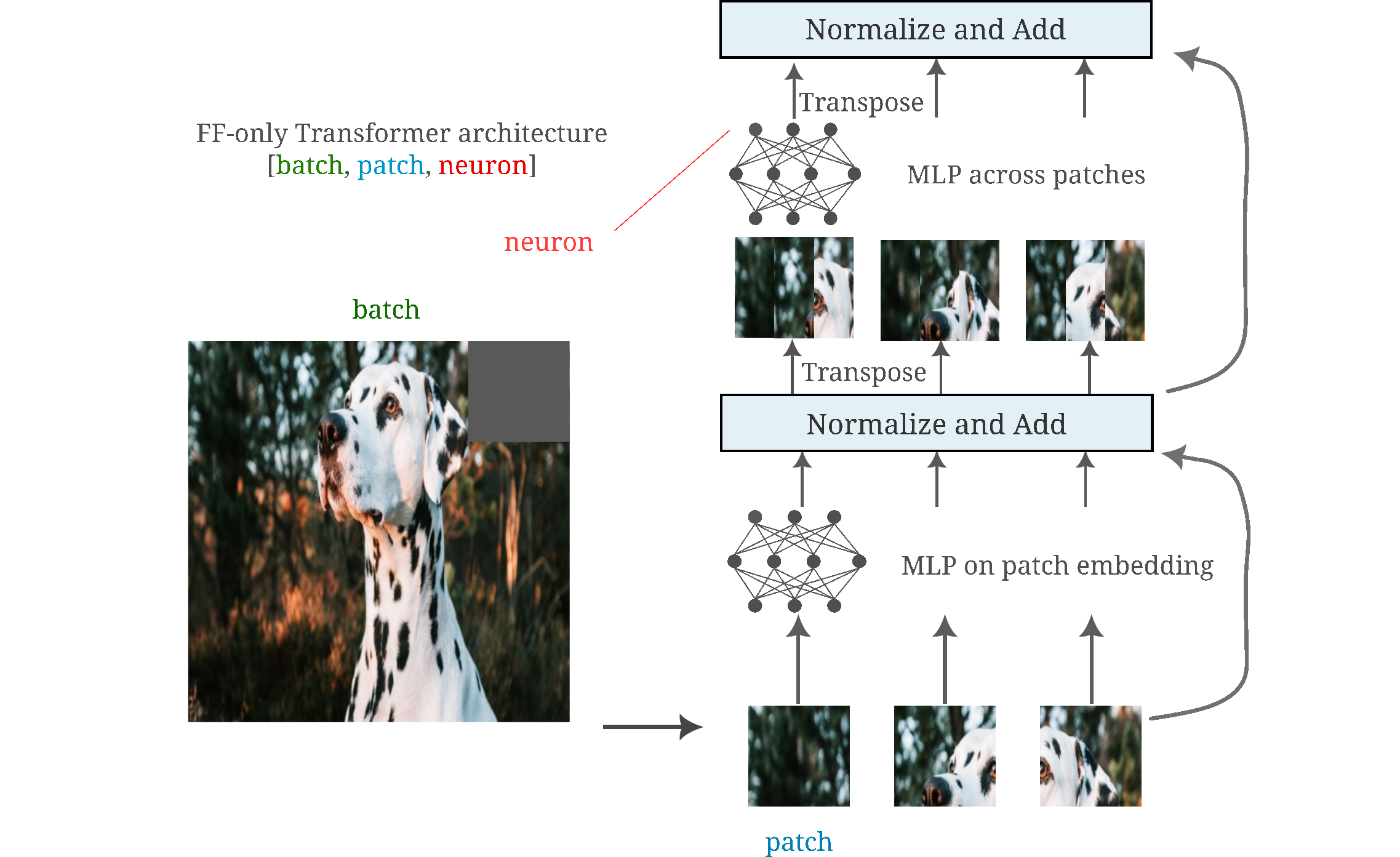
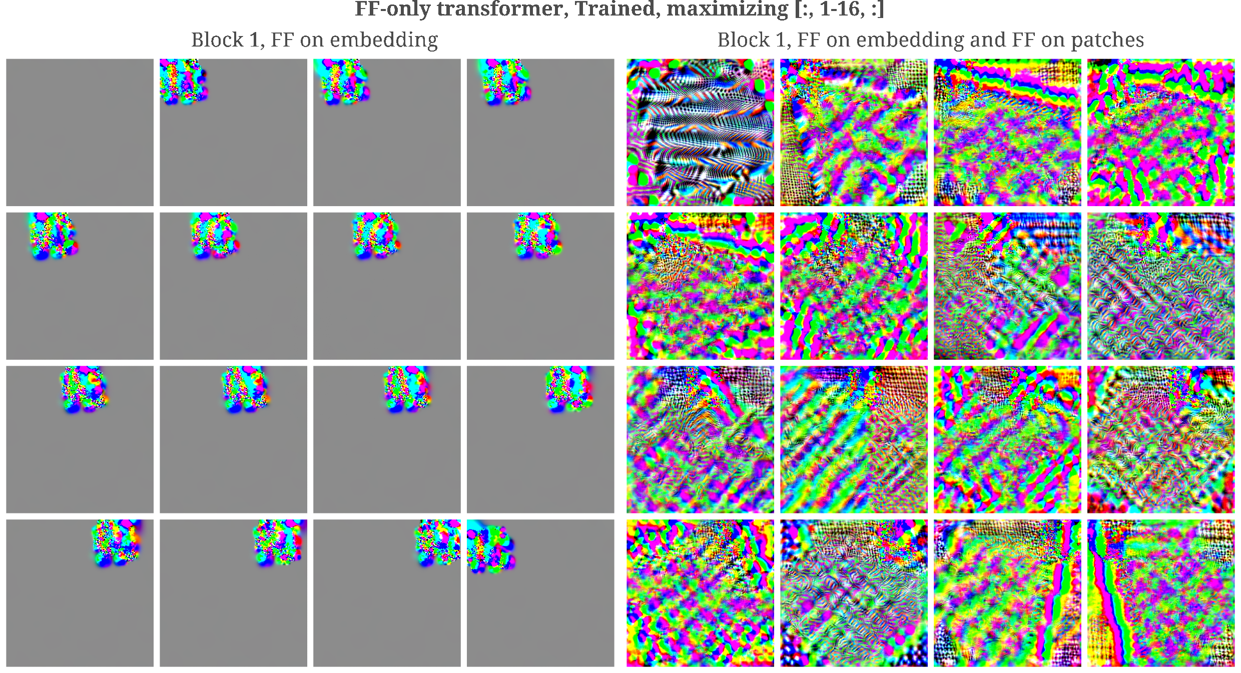
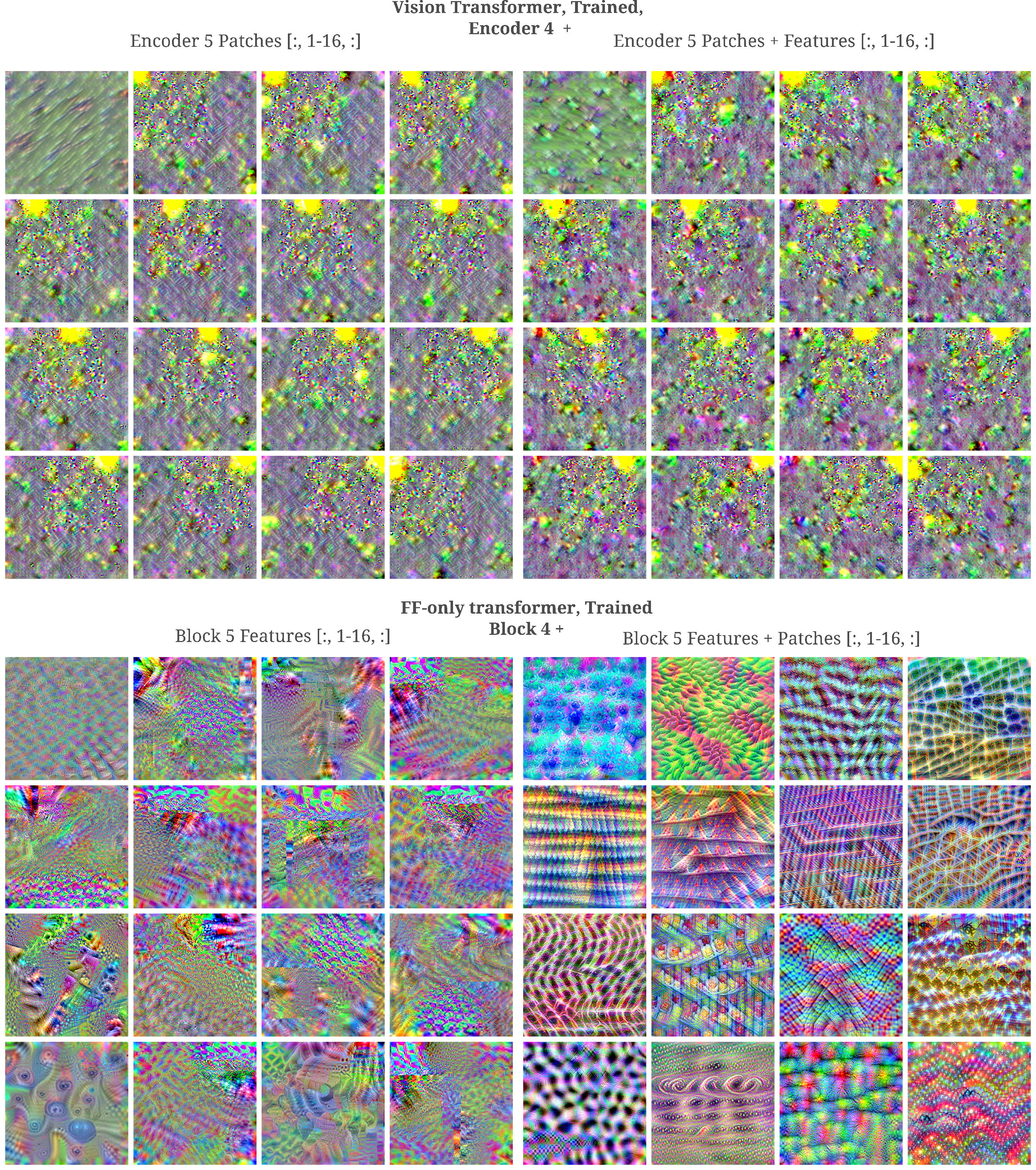
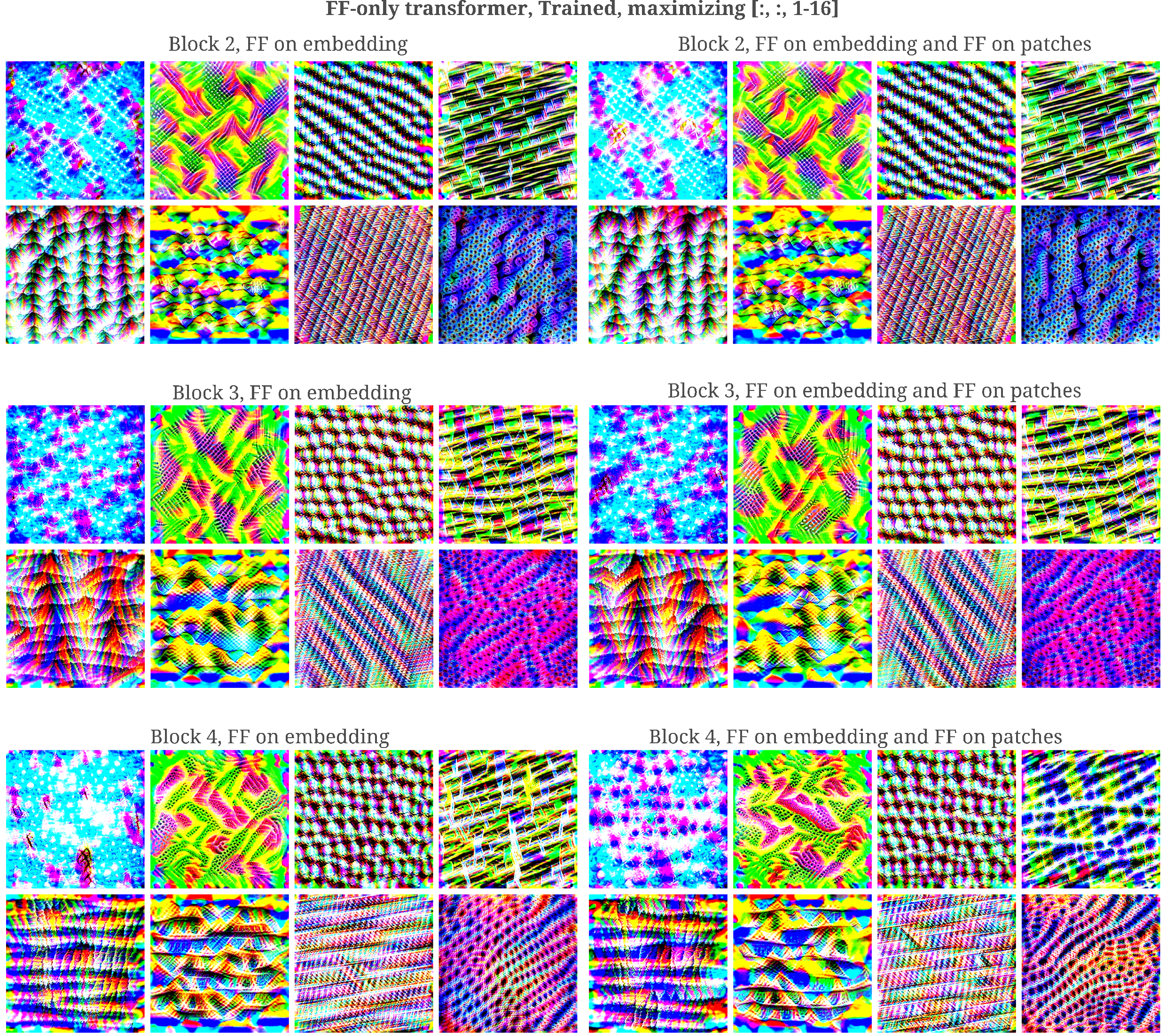
Thus far we have seen that we may recover feature maps from individual neurons of vision transformer encoder block outputs. It may be wondered if the same is true for attentionless transformers, introduced independently by Melas-Kyriazi and Tolstikhin. The model used on this page is that of Melas-Kyriazi, and may be found here.

These models do not use the attention operation to mix information between image patches but instead simply transpose the input and add a feed-forward layer (also called MLPs) applied to the embedding of each, followed by a second feed-forward layer across the patches. The order (mixing patches versus non-mixing layers) is therefore swapped compared to the ViT, and may be visualized as follows:

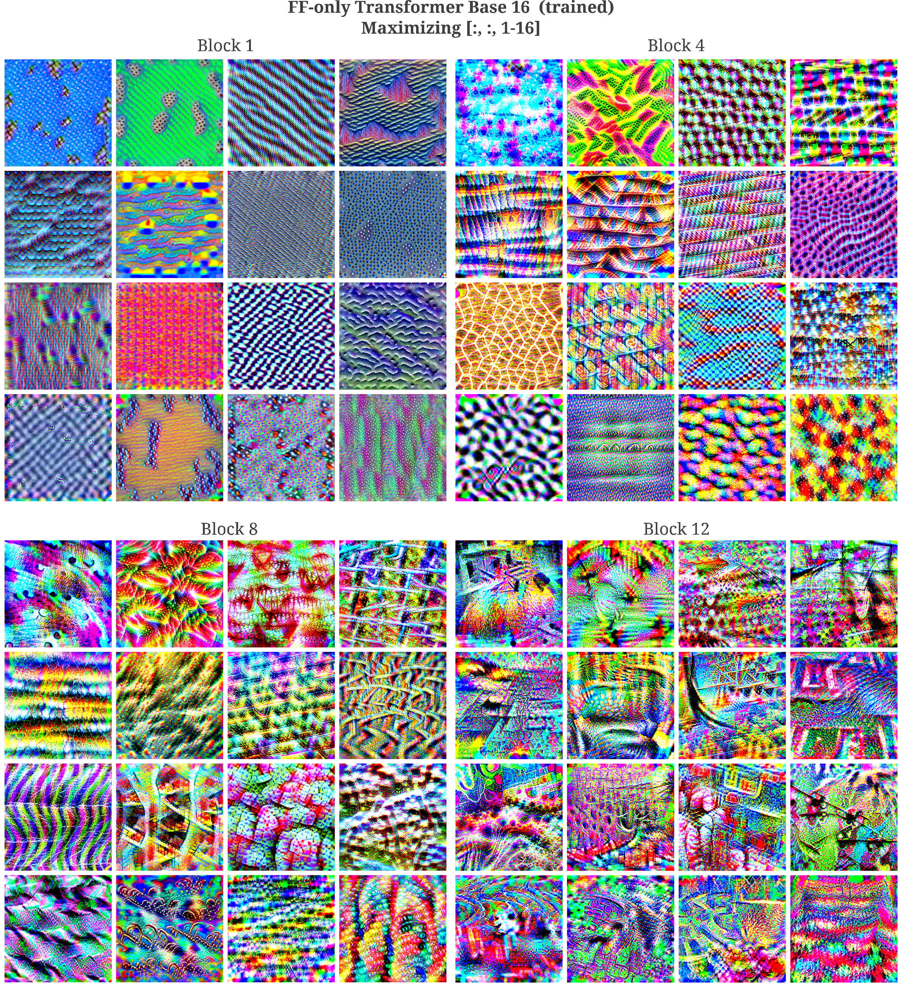
As for vision transformers, we find that these models form features in which each neuron of the block output is activated by a stereotypical pattern in early layers, and that this pattern becomes more abstract and complex the deeper the module in question. It is interesting to note that these neurons correspond to the output of the mixer layer whereas the block output features for the ViT correspond to the output of the non-mixing MLP in that model.

But there begin to be notable differences between vision transformers with attention layers and MLP mixers if we start to consider what a single neuron from a single patch focuses upon: as seen in the last section for ViTs, a neuron from a given patch will generally focus on the input region fed to that patch. For mlp mixers, however, we find that even in relatively shallow layers a neuron from a given patch typically focuses on the entirety of the input image, or else on a section of the image that does not correspond to the position of the patch in question.

This phenomenon can be most clearly seen in the following figure: observe how even at block 4 we find neurons in which it is impossible to know which patch they belong to without prior knowledge.

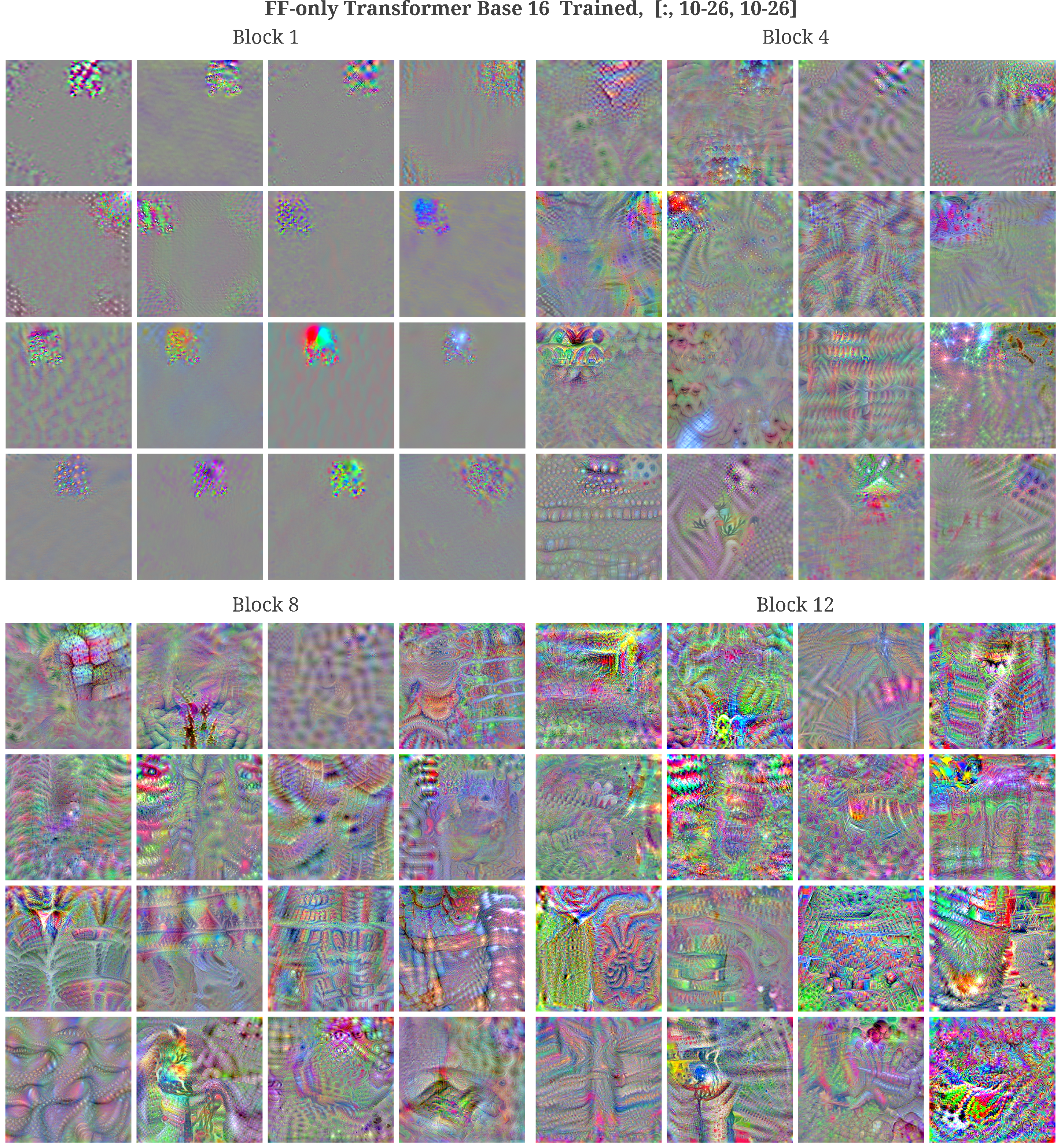
This suggests that the ‘Mixer’ is also an apt name for this architecture, being that the MLP-Mixer is apparently better at mixing information from different patches than the vision transformer is. We can assess this further by observing the ability of all neurons of certain patches to re-form an input image in mixers compared to ViTs.

Upon further investigation, it may be appreciated that this mixing occurs fairly thoroughly even in the first block:

and this is reflected in the change from a uniform pattern in the features of the first block’s embedding MLP to the composition of patterns present in the first block’s patch-mixing MLP.

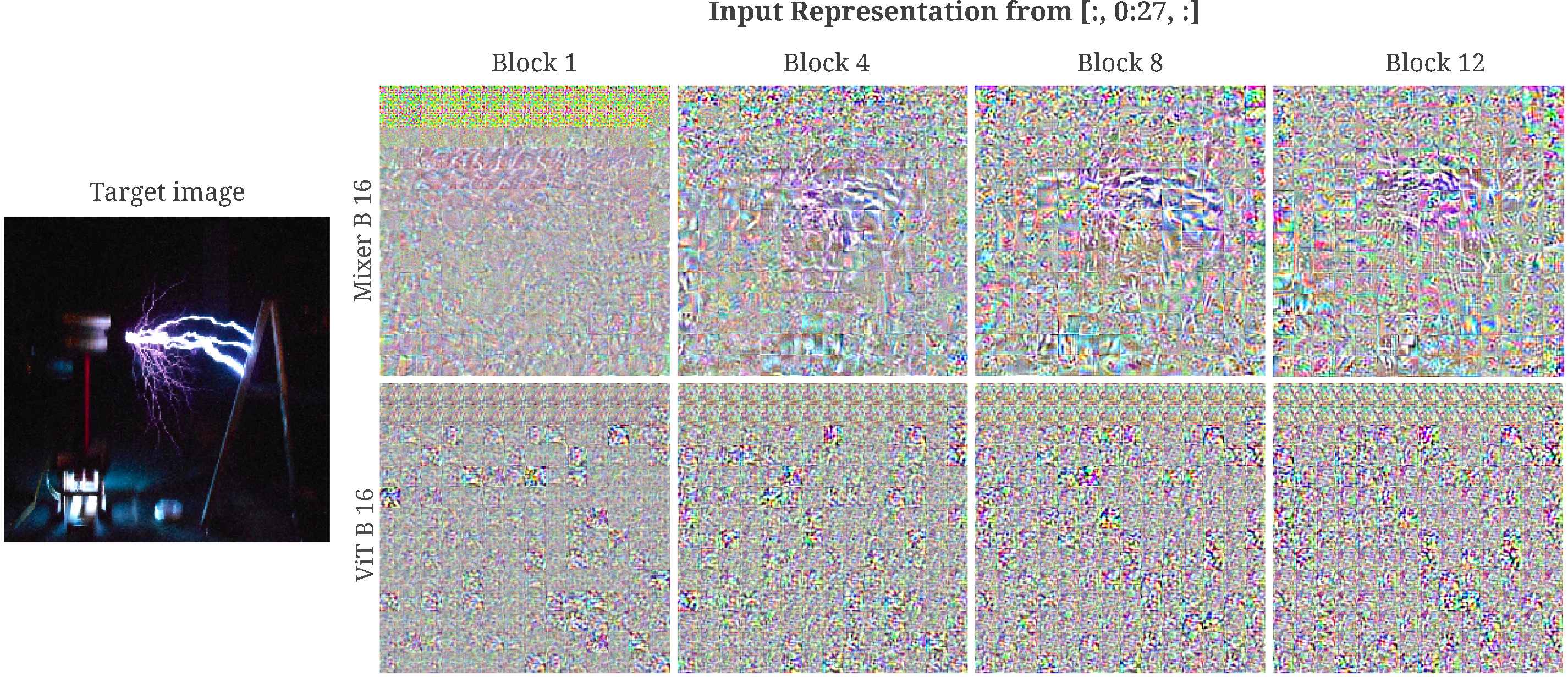
When the ability of the first 28 patches (approximately the first two rows for a 224x224 image) to re-create an input is tested, it is clearly seen that this subsection in mixers but not vision transformers are capable of representing an input to any degree of accuracy.

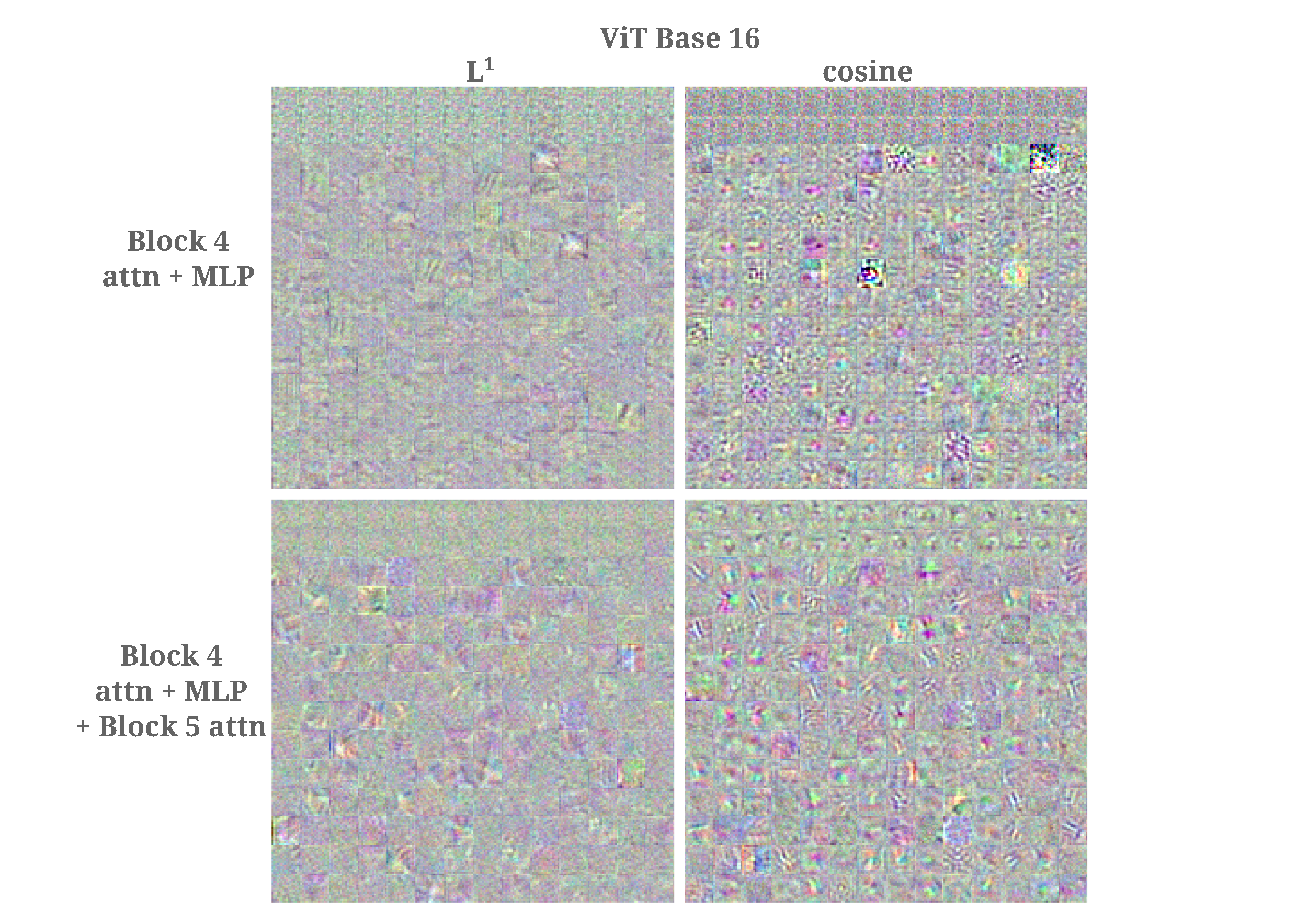
It may be wondered if this is due to a mismatch between the loss function we are minimizing (L1 distance) and the transformations that compose the self-attention layers of the transformer that are responsible for moving information from one patch to another. To recap, vision transformers typicaly use dot-product attention of some scaled version of the following in vector format

\[A(q, k, v) = \mathrm{softmax}(q \cdot k) v\]

or in matrix format,

\[A(Q, K, V) = (QK^T)V\]

The dot product may be thought of as combining information of relative vector magnitude and angle into one measure, and all information from the query token’s vector must pass through the dot product with the other token’s key and value vectors (or matricies). If one assumes that the fully connected layers that come after the self-attention layers in each transformer modules are capable of converting this angle-and-magnitude information into a pure distance (in vector space) information, it does not matter that we are optimizing $L^1$ or $L^2$ distance on this architecture.

But if there is some difficulty in converting between angle-and-magnitude and the difference norm, a more accurate representation may be found by optimizing for angle-and-magnitude instead. Here we focus on reducing the angle between the output of our generated input $O_l(a_g, \theta)$ and the layer’s output of the target input, $O_l(a, \theta)$. As above we take only the first 24 blocks of the output, so more accurately

Minimization of the angle betwen vectors can be done by finding the gradient of the generated input $a_g$ with respect to the cosine of the vector versions of $O(a_g, \theta)$ and $O(a, \theta)$ as follows:

\[\cos(O_l(a, \theta), O_l(a_g, \theta)) = \frac{O_l(a, \theta) \cdot O_l(a_g, \theta)}{|| O_l(a, \theta) ||_2 || O_l(a_g, \theta) ||_2} \\ a_{n+1} = a_n + \nabla_{a_n} (1 - \cos(O_l(a, \theta), O_l(a_g, \theta))\]

where we minimize the value $1 - \cos(\phi)$ because we want to minimize the angle between vectorized versions of the model’s output (and $\cos(\phi) = 1$ when $\phi = 0$).

Minimizing angle between target and generated input does lead to mixing of information between the first 24 and the other patches, however. Using the same target input as above, minimizing $\cos (\phi)$ results in poor representations, regardless of whether the output is taken as the MLP or as the dot product attention layer.

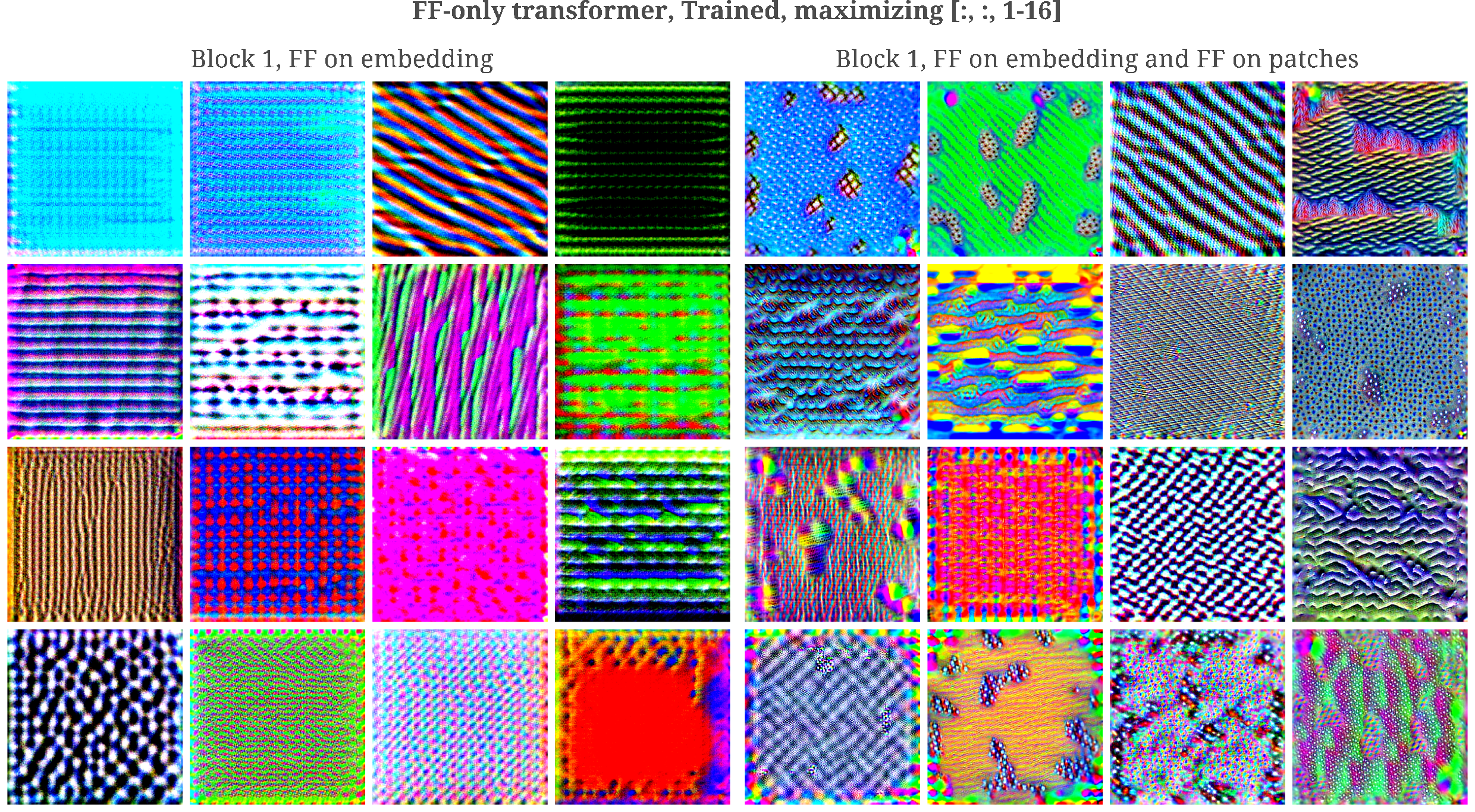
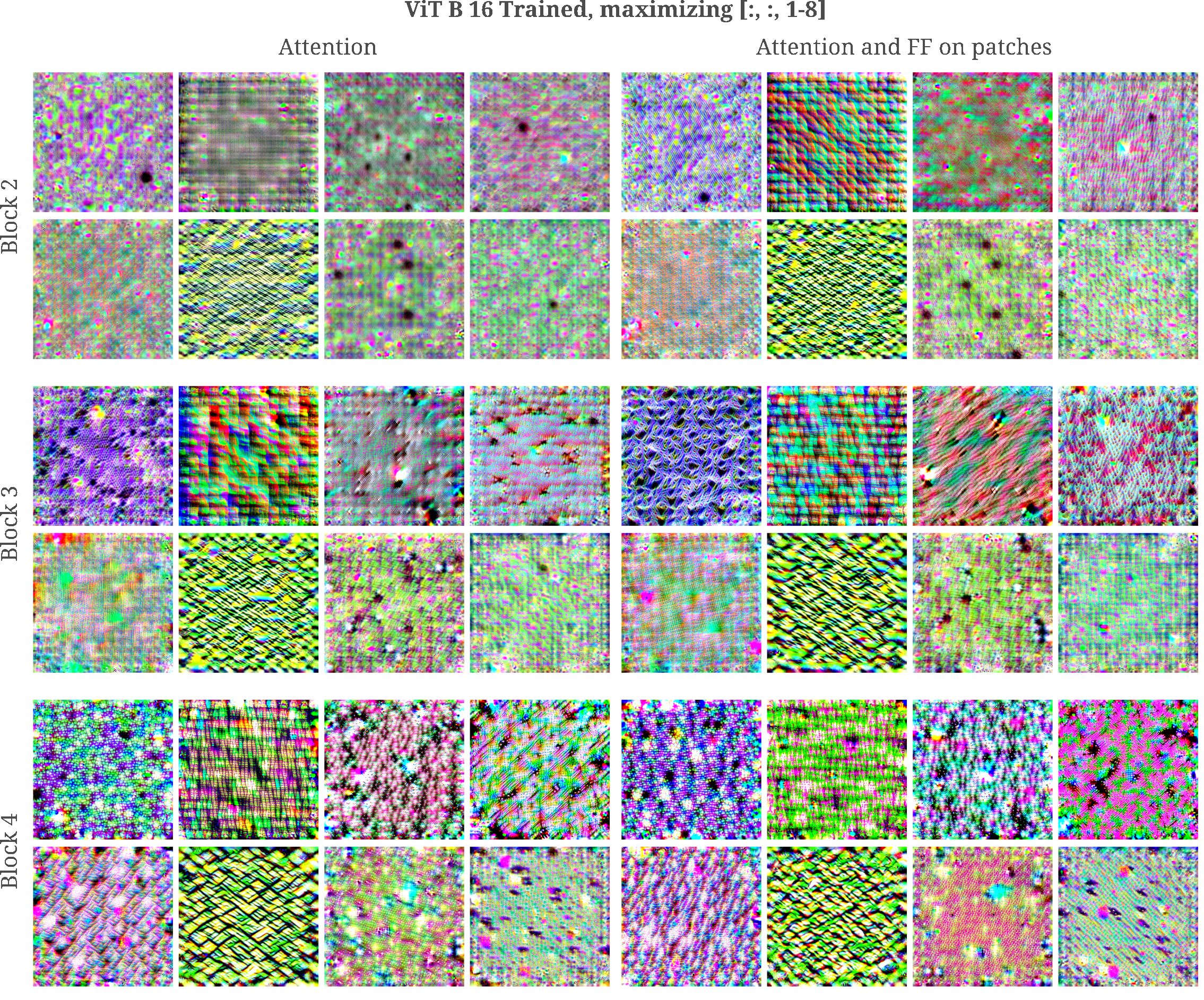
The superior mixing in the MLP mixer architecture compared to the vision transformer may also be observed by finding the feature maps of individual patches early in the model, maximizing activations of all elements of patch after an across-patch mixing layer (which occurs second for mixers and first for ViTs) or after the embedding dimension layer (first for mixers and second for ViTs).

There are two notable observations when we observe the features corresponding to a single input patch at one particular layer: first, there is very little difference between the patch and feature maps of the vision transformer compared to what is found for mixers, and second that the ViT primarily focuses on the input region corresponding the patch identity (note the bright yellow squares) whereas the mixer attends more broadly to the entire input, regardless of whether we observe mixer or embedding MLP layer activation.

On the other hand, when we observe the feature maps for neurons across all patches, there is less difference between then ViT and MLP-Mixer.

Deep Dream

Given some image, it may be wondered how a computer vision model would modify that image in order to increase the activation of some component of that model. This is similar to the feature visualization procedure used above but starts with a natural image rather than random noise.

For a trained ViT Base 32 we have the following: