Feature Visualization I: Feature Maps

Introduction

Suppose one wished to perform a very difficult task, but did not know how to begin. In mathematical problem solving, one of the strategies most commonly used to approach a seemingly impossible problem is to convert that problem into an easier one, and solve that. In many respects, the field of deep learning places the same importance on the ‘make it easier’ principle. Most problems faced by the field certainly fall into the category of being very difficult: object recognition, indeed, is so difficult that no one has made much progress in this problem by directly programming a computer with explicit instructions in decades. The mathematical function mapping an input image to its corresponding output classification is therefore very difficult to find indeed.

Classical machine learning uses a combination of ideas from statistics, information theory, and computer science to try to find this and other difficult functions in a limited number of steps (usually one). Deep learning distinguishes itself by attempting to approximate functions using more than one step, such that the input is represented in a better and better way before a final classification is made. In neural networks and similar deep learning approaches, this representation occurs in layers of nodes (usually called neurons).

As we will be employing a model whose hidden layers consists primarily of 2-dimensional convolutions, first it may be beneficial to orient ourselves to the layout of a standard example of this type of layer. See this page for a recap of what a convolution is and why this operation is so useful for deep learning models dealing with images.

For a convolutional layer with a single kernal, the output is a two-dimensional grid corresponding to the value of the convolutional operation centered on each of the pixels. Therefore it could be expected that an image of 256 pixels by 256 pixels, ie a 256x256 tensor with each pixel intensity value corresponding to one tensor element, when passed through a convolutional layer will give an output tensor of 256 by 256 (if a specific type of padding is used to deal with edge pixels). There are normally multiple kernals used per convolutional layer, so for a layer with say 16 kernals (also called ‘filters’) we would have a 16x256x256 output. Each of the 16 elements are referred to as a ‘feature map’, and on this page will always precede the other tensor elements.

Feature Visualization from First Principles

The process of sequential input representation, therefore, is perhaps the defining feature of deep learning. This representation does make for one significant difficulty, however: how does one know how the problem was solved? We can understand how the last representation was used to make the output in a similar way to how other machine learning techniques give an output from an input, but what about how the actual input is used? The representations may differ significantly from the input itself, making the general answer to this question very difficult.

One way to address this question is to try to figure out which elements of the input contribute more or less to the output. This is called input attribution.

Another way is to try to understand what the representation of each layer actually respond to with regards to the input, and then try to understand how this response occurs. Perhaps the most natural way to study this is to feed many input into the model and observe which input give a higher activation to any layer or neuron or even subset of neurons across many layers, and which images yield a lower activation.

There is a problem with this approach, however: images as a rule do not contain only one characteristic that could become a feature, and furthermore even if some did there is little way of knowing how features would be combined together between layers being that nonlinear transformations are applied to all layers in a typical deep learning model.

Instead we can approach the question of what each neuron, subset of neurons, or layer responds to by having the neurons in question act as if they are our model’s outputs, and performing gradient ascent on the input. We have seen elsewhere that an output can effectively specify the expected image on the input using gradient ascent combined with a limited number of priors that are common to nearly all natural images (pixel correlation, transformational resiliency, etc.) so it is logical to postulate that the same may be true for outputs that are actually hidden layers, albeit that maximizing the activation of a hidden layer neuron or layer does not have an intrinsic meaning w.r.t the true output.

To make this more precise, what we are searching for is an input $a’$ such that the activation of our chosen hidden layer or neuron $z^l$ (given the model configuration $\theta$ and input $a$) denoted by $z^l(a, \theta)$ is maximized,

\[a' = \underset{a}{\mathrm{arg \; max}} \; z^l(a, \theta)\]

Convolutional layers typically have many feature maps, each specified by a separate set of parameters. We will mostly focus on finding inputs $a’$ that maximally activate a single feature, rather than all features for a layer given that there may be hundreds of features per layer. For a two-dimensional convolutional layer with $m$ rows and $n$ columns, the total activation $z$ at layer $l$ for feature $f$ is denoted

\[z^l_f = \sum_m \sum_n z^l_{f, m, n}\]

In tensor notation, this would be written as the total activation of the tensor [f, :, :] where : indicates all elements of the appropriate index.

For a subset of neurons in layer $l$ and feature $f$, the total activation of all neurons in row $n$, denoted

\[z^l_{f, m} = \sum_n z^l_{f, m, n}\]

which is denoted as the sum of the elements of the tensor [f, m, :]. The element of row m and column n is denoted of feature f is [f, m, n].

Finding the exact value of $a’$ can be very difficult for non-convex functions like hidden layer outputs. An approximation for the input $a’$ such that when given to our model gives an approximate maximum value of $z^l_f(a’, \theta)$ may be found via gradient descent. The gradient in question used on this page is the gradient of the $L_1$ metric between a tensor with all values equal to some large constant $C$ and the tensor activation of a specific layer and feature (or a subset of this layer) $z^l_f$

\[g = \nabla_a (C - z^l_f(a, \theta))\]

For an example, if we were to optimize a feature comprising two neurons then the gradient would be taken as the $L^1$ distance between the activations of neurons $f_1, f_2$ and the point $C, C$, which is $(C - f_1) + (C - f_2)$. Miminization of an $L^1$ distance between a feature’s activation and some constant is one among many ways one could possibly maximize a feature’s activations, but will be the primary method discussed here.

At each step of the gradient descent procedure, the input at point $a_k$ is updated to make $a_{k+1}$ as follows

\[a_{k+1} = a_k - \epsilon * g_k\]

with $*$ usually denoting broadcasted multiplication from scalar $\epsilon$ to tensor $g_k$. The hope is that the sequence $a_k, a_{k+1}, a_{k+2}, …, a_j$ converges to $a’$, which happily is normally the case for appropriately chosen values of $\epsilon$ for most layers.

We will be using Pytorch for our experiments on this page. As explained elsewhere, Pytorch uses symbol-to-number differentiation as opposed to symbol-to-symbol differentiation which means that the automatic differentiation engine must be told which gradients are to be computed before forward propegation begins. Practically speaking, this means that getting the gradient of a model’s parameters with respect to a hidden layer is difficult without special methods.

Rather than deal with these somewhat tricky special functions, we can instead simply modify the model in question in order to make whichever layer is of interest to be our new output. This section will focus on the InceptionV3 model, which is as follows:

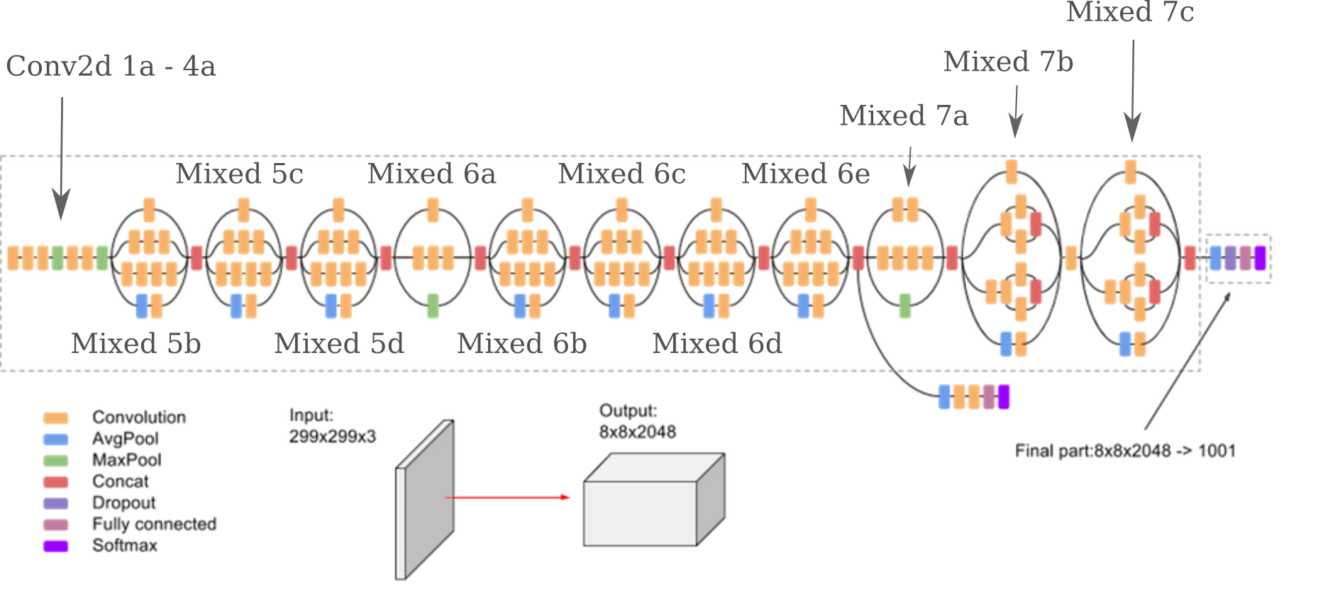
(image retrieved and modified from Google docs)

and may be found on the following github repo. Inspecting this repository will show us how the inceptionv3 model has been implemented, and that there are a few differences between the origina model and the open-source Pytorch version (most notably that the last layers do not contain softmax layers by default).

A pre-trained version of InceptionV3 may be loaded from torch.hub

Inception3 = torch.hub.load('pytorch/vision:v0.10.0', 'inception_v3', pretrained=True).to(device)

And after deciding on which layer is of interest, the model may be modified by writing a class that takes the original InceptionV3 model as an initialization argument and then specifies what to do with the layers in question. As this is a pre-trained model, it generally does not make sense to change the configuration of the layers themselves but we can modify the model to output any layer we wish. Here we want to view the activations of theConv2d_3b_1x1 layer

class NewModel(nn.Module):

	def __init__(self, model):
		super().__init__()
		self.model = model

	def forward(self, x):
		# N x 3 x 299 x 299
		x = self.model.Conv2d_1a_3x3(x)
		# N x 32 x 149 x 149
		x = self.model.Conv2d_2a_3x3(x)
		# N x 32 x 147 x 147
		x = self.model.Conv2d_2b_3x3(x)
		# N x 64 x 147 x 147
		x = self.model.maxpool1(x)
		# N x 64 x 73 x 73
		x = self.model.Conv2d_3b_1x1(x)
		return x

and because we are taking the original trained model as a parameter, each layer maintains its trained weight and bias.

Instantiating this model with the original InceptionV3 model object

newmodel = NewModel(Inception3)

we can now use our newmodel class to find the activation of the Conv2d_3b_1x1 layer and perform backpropegation to the input, which is necessary to find the gradient of the output of this layer with respect to the input image.

To be specific, we want to find the gradient of the output of our layer in question $O^l$ with respect to the input $x$

\[g = \nabla_a O^l(a, \theta)\]

def layer_gradient(model, input_tensor, desired_output):
  ...
	input_tensor.requires_grad = True
	output = model(input_tensor).to(device)
	focus = output[0, 200, :, :] # the target to maximize the output
	target = torch.ones(focus.shape).to(device)*200 # make a large target of the correct dims
	loss = torch.sum(target - focus)
	loss.backward()
	gradient = input_tensor.grad
	return gradient

Now that we have the gradient of the output (which is our hidden layer of interest in the original InceptionV3 model) with respect to the input, we can perform gradient descent on the input in order to maximize the activations of that layer. Note that this process is sometimes called ‘gradient ascent’, as we are modifying the input in order to maximize a value in the output. But as our loss is the $L_1$ distance from a tensor with all elements assigned to be a large constant $C=200$, gradient descent is the preferred terminology on this page as this loss is indeed minimized by moving against the gradient.

For this page These restrictions may be thought of as Bayesian priors that we introduce, knowing certain characteristics that natural images possess. The three characteristics that are implemented below are relative smoothness (enforced by Guassian convolution via torchvision.transforms.functional.gaussian_blur) and transformational invariance (using torchvision.transforms.Resize()).

We can use this procedure of gradient descent on the input combined with priors to visualize the input generated by maximizing the output of the given neuron, or layer. If we choose module mixed_6b and maximize the activations of neurons in the 654th (of 738 possible) feature map of this module, we find an interesting pattern is formed.

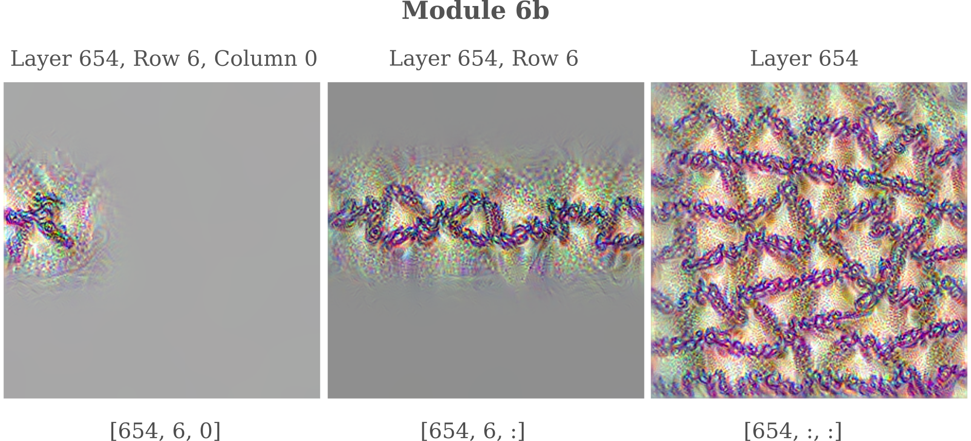
The first thing to note is that the tensor indicies for ‘row’ and ‘column’ do indeed accurately reflect the position of the pixels affected by maximization of the output of the neuron of a given position.

It is interesting to consider how exactly the feature pattern forms from tiles of each row and column’s contribution. For each feature map in module mixed_6b, we have a 17x17 grid and can therefore iterate through each element of the grid, left to right and top to bottom, like reading a book. Slicing tensors into non-rectangular subsets can be difficult, so instead the process is to compose the loss of two rectangular slices: one for all columns of each row preceding the current row, and another rectangle for the current row up to the appropriate column.

def layer_gradient(model, input_tensor, desired_output, index):
	...
	input_tensor.requires_grad = True
	output = model(input_tensor).to(device)
	row, col = index // 17, index % 17
	if row > 0:
		focus = output[0, 415, :row, :] # first rectangle of prior rows
		focus2 = output[0, 415, row, :col+1] # second rectangle of the last row
		target = torch.ones(focus.shape).to(device)*200
		target2 = torch.ones(focus2.shape).to(device)*200
		loss = torch.sum(target - focus)
		loss += torch.sum(target2 - focus2) # add losses

	else:
		focus = output[0, 415, 0, :col+1]
		target = torch.ones(focus.shape).to(device)*200
		loss = torch.sum(target - focus)

	loss.backward()
	gradient = input_tensor.grad
	return gradient

Note that we must also set our random seed in order to make reproducable images. This can be done by adding

seed = 999
random.seed(seed)
torch.manual_seed(seed)

to the function that is called to make each input such that the above code is processed before every call to layer_gradient().

One important note on reproducing a set seed: the above will not lead to reproducibility (meaning identical outputs each time the code is run) using Google Colab. For reasons that are not currently clear, image generation programs that appropriately set the necessary random seeds (as above) yield identical output images each time they are run on a local machine, but different output images each time they are run on Colab. Preliminary observations give the impression that this issue is not due to incorrect seed setting but rather some kind of round-off error specific to Colab, but this has not been thoroughly investigated.

Running our program on a local machine to enforce reproducibility between initializations, we have

We come to an interesting observation: each neuron when optimized visibly affects only a small area that corresponds to that neuron’s position in the [row, col] position in the feature tensor, but when we optimize multiple neurons the addition of one more affects the entire image, rather than the area that it would affect if it were optimized alone. This can be seen by observing how the rope-like segments near the top left corner continue to change upon addition of neurons that alone only affect the bottom-right corner.

How is this possible? Neurons of any one particular layer are usually considered to be linearly independent units, and assumption that provides the basis for being able to apply the gradient of the loss to each element of a layer during training. But if the neurons of layer mixed_65 654 were linearly independent with respect to the input maps formed when optimizing these neuron’s activations, we would not observe any change in areas unaffected by each neuron. It is at present not clear why this pattern occurs.

For the 415th feature map of the same module, a somewhat more abstract pattern is formed. Observe how a single neuron exhibits a much broader field of influence on the input when it is optimized compared to the previous layer: this is a common feature of interior (ie not near layer 0 or 738) versus exterior (close to 0 or 748 in this particular module). This is likely the result of differences in the inception module’s architecture for different layers that have been concatenated to make the single mixed_6b output.

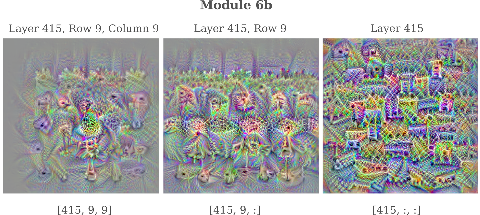
Something interesting to note is that the neuron at position $[415, 9, 9]$ in the mixed_6b module is activated by a number of different patterns at once, which is notably different than the neuron at position $[354, 6, 0]$ which is maximally activated by one rope-like pattern alone.

The approach detailed above for introducing transformational invariance leads to fairly low-resolution images by design (which allows for less time to be taken while generating an image). The octave method increases resolution and clarity at the expense of more time per image generated, and may be implemented as follows:

def octave(single_input, target_output, iterations, learning_rates, sigmas):
	...
	start_lr, end_lr = learning_rates
	start_sigma, end_sigma = sigmas

	for i in range(iterations):
		single_input = single_input.detach() # remove the gradient for the input (if present)
		input_grad = layer_gradient(Inception, single_input, target_output) # compute input gradient
		single_input -= (start_lr*(iterations-i)/iterations + end_lr*i/iterations) * input_grad # gradient descent step
		single_input = torchvision.transforms.functional.gaussian_blur(single_input, 3, sigma=(start_sigma*(iterations-i)/iterations + end_sigma*i/iterations)) # gaussian convolution

	return single_input

This function may now be called to perform gradient descent with scaling, and in the following method three octaves are applied: one without upscaling, one that scales to 340 pixels, and one that scales to 380.

def generate_singleinput(model, input_tensors, output_tensors, index, count, random_input=True):
	...
	single_input = octave(single_input, target_output, 100, [0.4, 0.3], [2.4, 0.8])
 
	single_input = torchvision.transforms.Resize([340, 340])(single_input)
	single_input = octave(single_input, target_output, 100, [0.3, 0.2], [1.5, 0.4])

	single_input = torchvision.transforms.Resize([380, 380])(single_input)
	single_input = octave(single_input, target_output, 100, [0.2, 0.1], [1.1, 0.3])

The images produced are of higher resolution and are generally clearer than with only down-sampling used, so most of the rest of the images on this page are generated via gradient descent with octaves.

It is worth assessing how representative the images produced using octaves and Gaussian convolutions with gradient descent are to the images produced with gradient descent alone. If the resulting images are completely different, there would be limited utility in using octaves to understand how features recognize an input. For four arbitrarily chosen features of module Mixed 6b, plotting pure gradient descent compared to octave-based gradient descent is as follows:

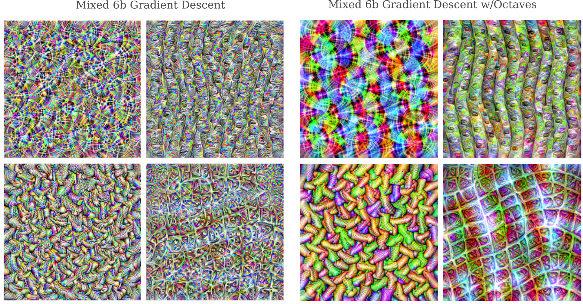
The images are clearly somewhat different, but the qualitative patterns are more or less unchanged. These results have been observed for features in other layers as well, providing the impetus for proceeding with using octaves and Gaussian convolutions with gradient descent to optimize the layers in images on the rest of the page.

We can observe the process of generating an image using this octave method by plotting the average activation for each feature in a layer of interest, while attempting to maximize the total activation of some given feature. Maximizing the total activation of GoogleNet’s Feature 5 of Layer 5a (denoted in red) and plotting the average activation for all features of Layer 5a,

It is apparent that the process of maximizing the total activation of a given feature does not lead the others unchanged. In particular, a feature near 350 has an average activation that is only slightly less than the activation of the target feature. What this means is that an image that is optimized for activating feature 5 inadvertently activates this other feature as well, meaning that these are in a sense similar features. Using this method it is possible to map how similar each feature is from each other.

Mapping InceptionV3 Features

In the pioneering work on feature visualization in the original Googlenet architecture (aka InceptionV1), Olah and colleagues observed an increase in the complexity of the images resulting from maximizing the activation of successive layers in that model: the deeper into the network the authors looked, the more information could be gleaned from the input after performing gradient descent to maximize the layer’s activation. Early layers show maze-like patterns typical of early convolutional layers, which give way to more complicated patterns and textures and eventually whole objects. Curiously, the last layers were reported to contain multiple objects jumbled together, a phenomenon this author has observed elsewhere.

The InceptionV3 architecture differs somewhat from the GoogleNet that was thoroughly explored, so it is worth investigating whether or not the same phenomenon is observed for this model as well. To orient ourselves, the module map for the InceptionV3 model may be divided into four general regions.

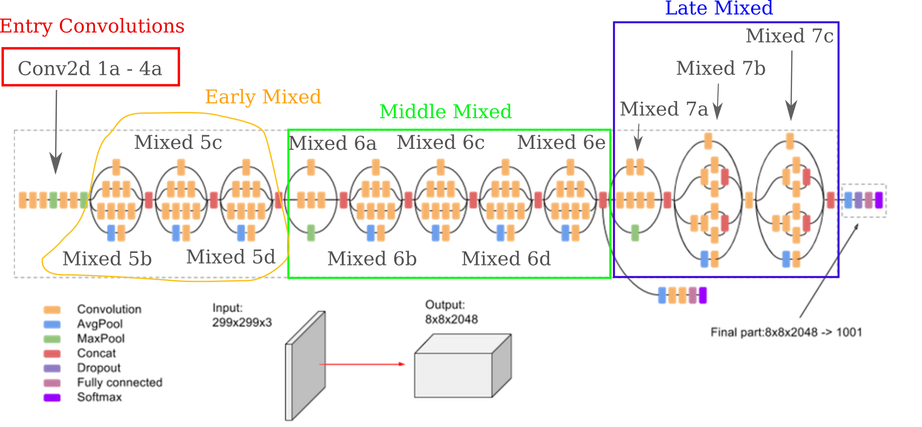
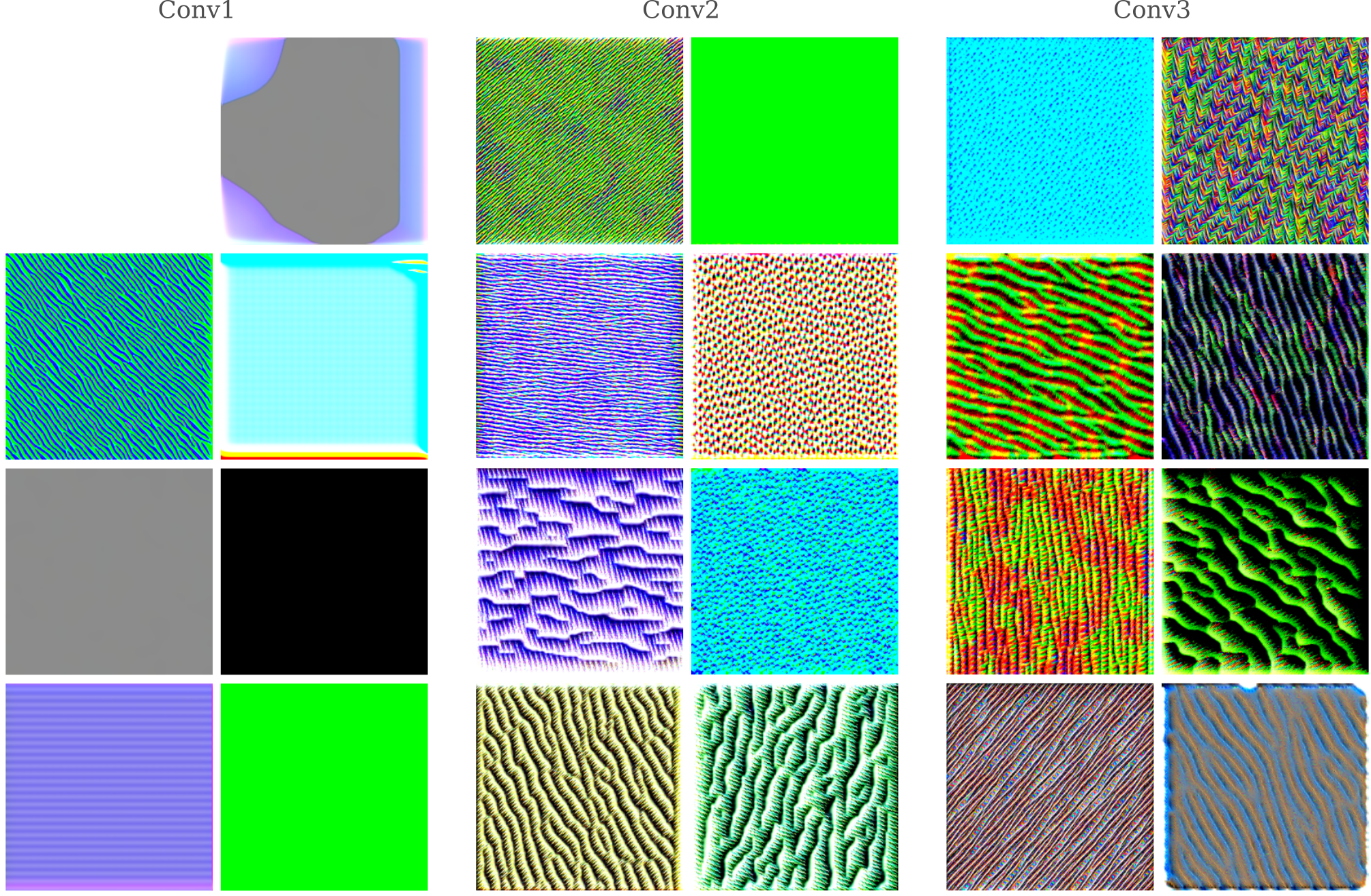
In the first of these regions, convolutions are applied in a sequential manner with no particularly special additions. Optimizing the first 16 features of each layer, we have

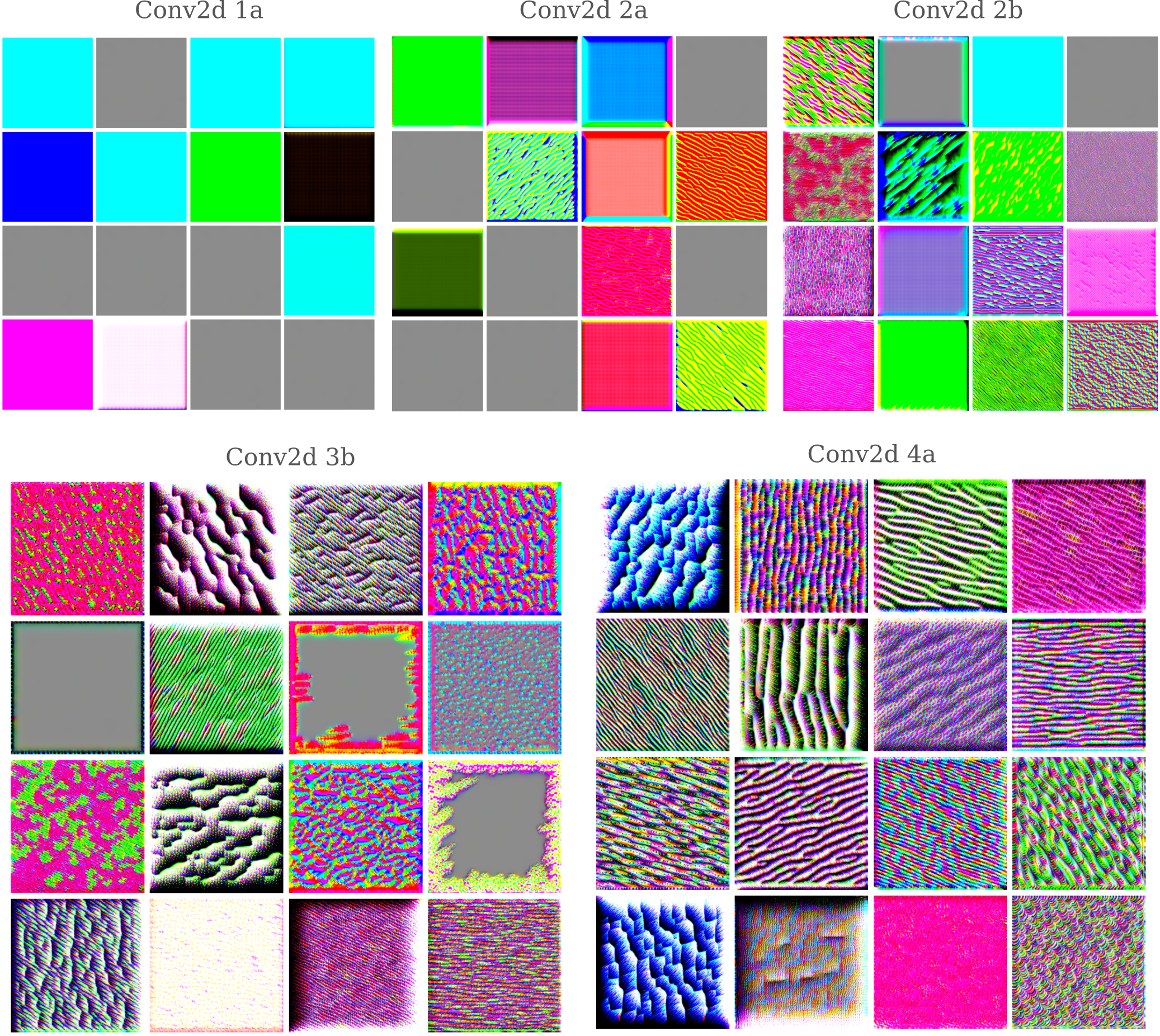
It is interesting to note that there are few in the input when we optimize for activation of the Conv2d 1a layer. Instead, it appears that the InceptionV3 network has learned a modified version of the CMYK color pallate, in which yellow has been substituted for a combination of yellow and blue (ie green). To this author’s knowledge it has not been found previously that a deep learning model has learned a color pallate, so it is unknown whether or not this behavior is specific to Inceptionv3. It should be noted that if optimization occurs without the octave process, similar colors are observed but a fine grid-like pattern reminiscent of CRT video appears for a minority of features.

Note that the gray filters signify a lack of gradient in that feature with respect to the input.

The second convolutional layer begins to respond to patterns in the image, and in the following layers the features become more detailed.

Next we come to the mixed convolutional layers, which are composed of modules (sometimes called inception units) that contain convolutional layers in parallel, which become concatenated together at the end of the module to make one stack of the features combining all features from these units. The first three mixed units have been somewhat arbitrarily classified as ‘early mixed’. Optimizing the activation of 8 features from each layer,

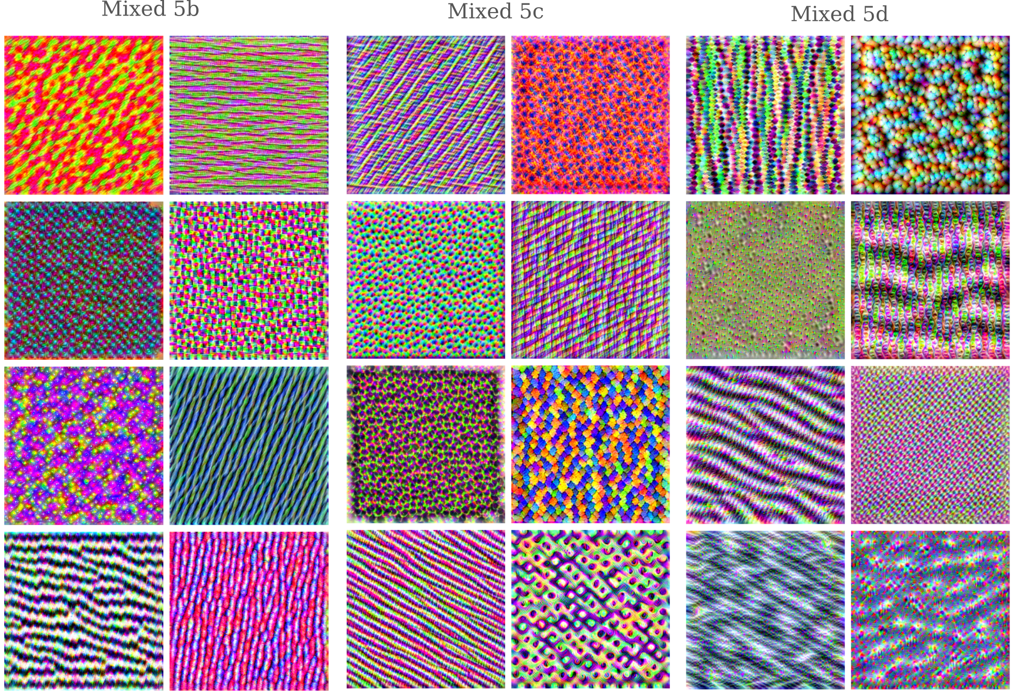
It is clear that more complicated patterns are found when we visualize the features that these early mixed layers respond to.

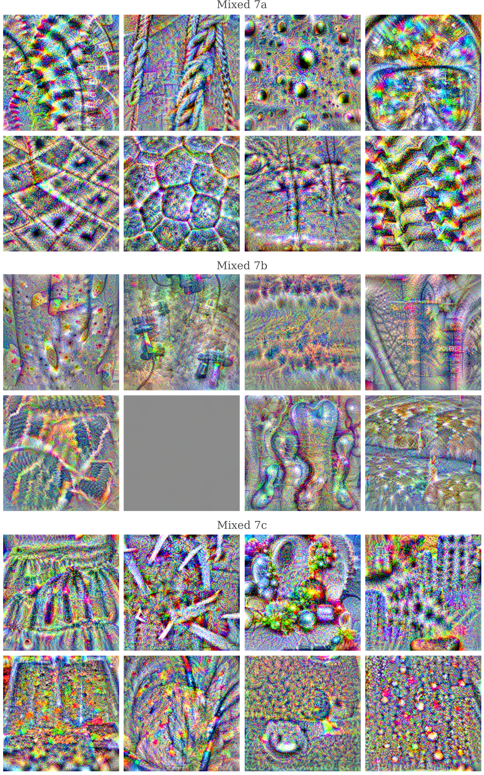
At the middle mixed layers, we start to see more distinctive shapes appear in a minority of features, with the rest usually forming complicated patterns. The following figure plots the first 8 features per layer denoted:

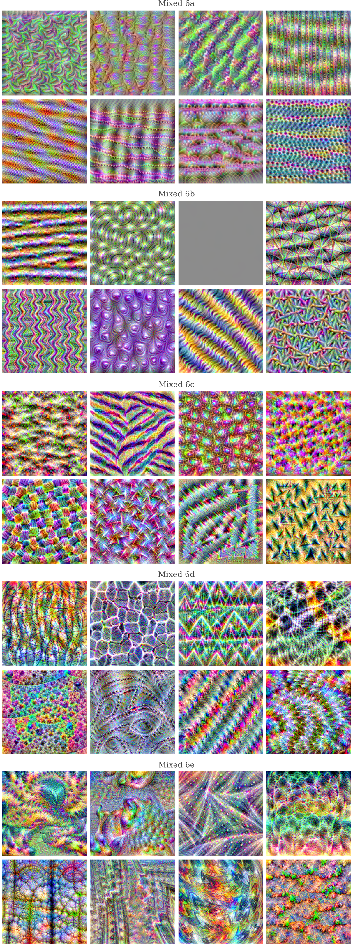
Observe the animal eyes generated by the second feature of layer Mixed 6b, or what appears to be a porcupine in the second feature of layer Mixed 6e.

In the late mixed layers, feature activation optimization often leads to recognizable shapes being formed. For example, the second feature of layer Mixed 7a is a rope harness, and the fourth feature of the same layer appears to be a snorkeling mask. But note also how may colors are mixed together, and sometimes many shapes as well.

Feature Maps are Metric Invariant

It may be wondered how specific these feature maps are to the optimization process, and in particular whether minimization of different metrics between the feature activations $z^l_f$ and $C$ lead to different feature maps. This is equivalent to wondering whether instead of maximizing the total activation ($L^1$ metric), we instead weight the maximization of smaller elements higher compared to maximization of larger elements of $z^l_f$ (corresponding to the $L^2$ metric) or else find use the metric with the largest absolute value, $L^\infty$.

Focusing on mapping features from InceptionV3 layer Mixed 6b, we optimize the input using the $L^2$ metric of the distance between the feature’s activations and some large constant,

loss = 5*torch.sqrt(torch.sum((target-focus)**2))

as well as the $L^\infty$ metric of that same distance, which can be implemented as follows:

loss = torch.linalg.norm((target-focus), ord=np.inf)

For the first four features of InceptionV3’s layer Mixed 6b, we can see that the same qualitative objects and patterns are formed regardles of the metric used. Note, however, that in general the $L^1$ metric has the smallest amount of high-frequency noise in the final image and is therefore preferred.

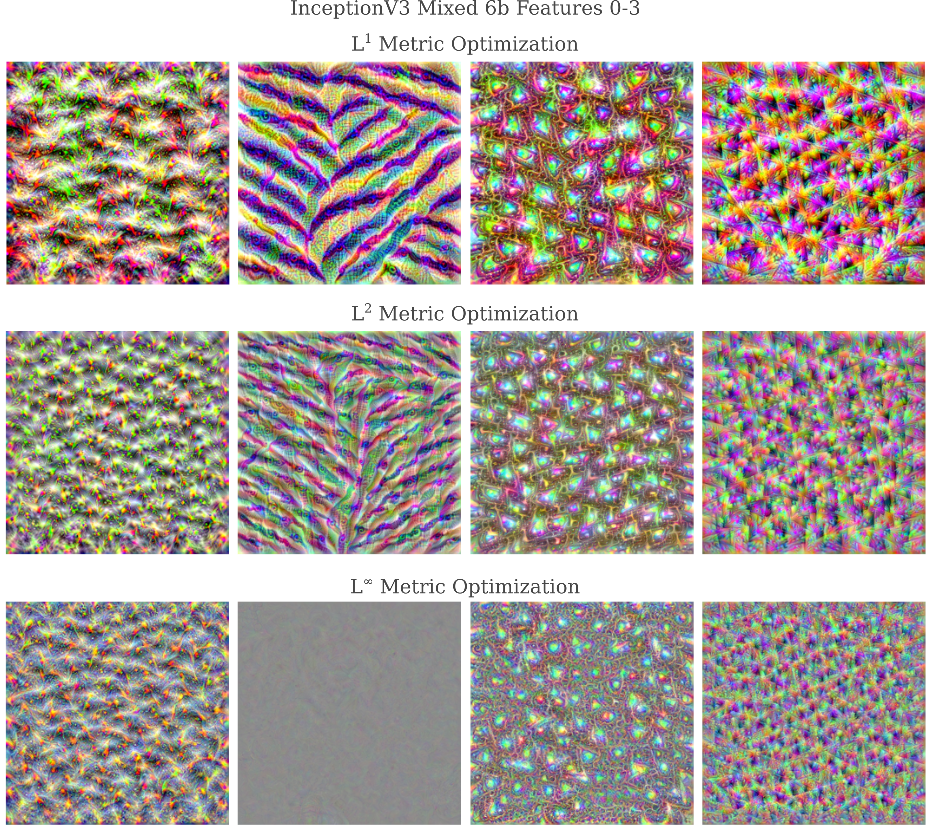
In conclusion, the feature maps presented here are mostly invariant with respect to the specific measurement used to determine how to maximize the feature activations.

Mapping GoogleNet Features

In another article, we saw how there were differences between how recognizable a generated input representative of a certain ImageNet training class was between various neural networks. In particular, InceptionV3 generally yielded less-recognizable images than GoogleNet. This brings about the question of whether or not the feature maps in the previous section might also be less recognizable than those for GoogleNet, and this can be easily explored.

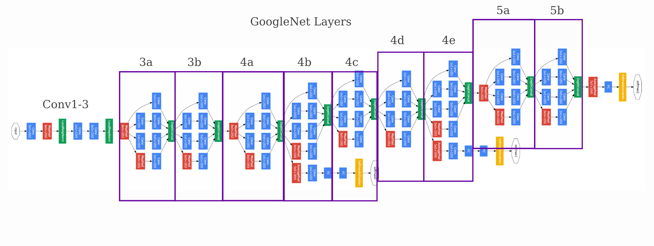
To recap, GoogleNet was the first published model to use the Inception architecture in which different convolutional layers are made in parallel before being joined. GoogleNet is only about half as deep as InceptionV3, and has the following architecture (layer names modified for clarity):

Initializing our model with an implementation of GoogleNet trained on ImageNet

model = torch.hub.load('pytorch/vision:v0.10.0', 'googlenet', pretrained=True, init_weights=True).to(device)

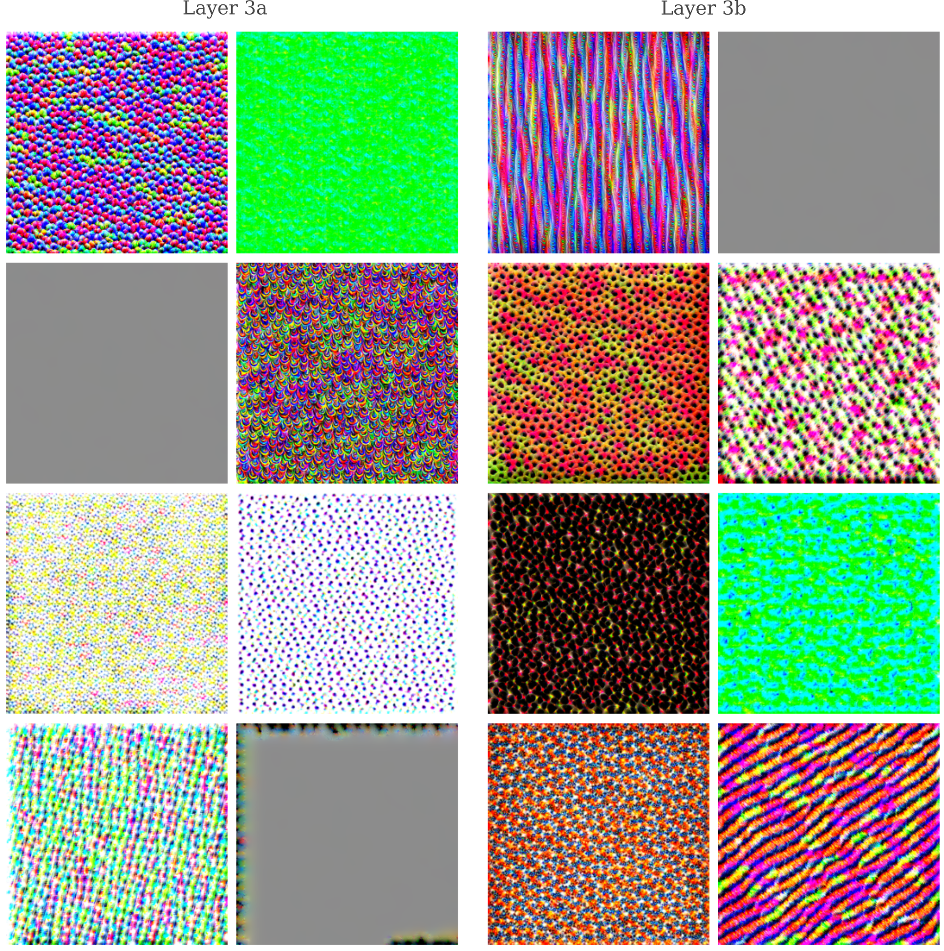
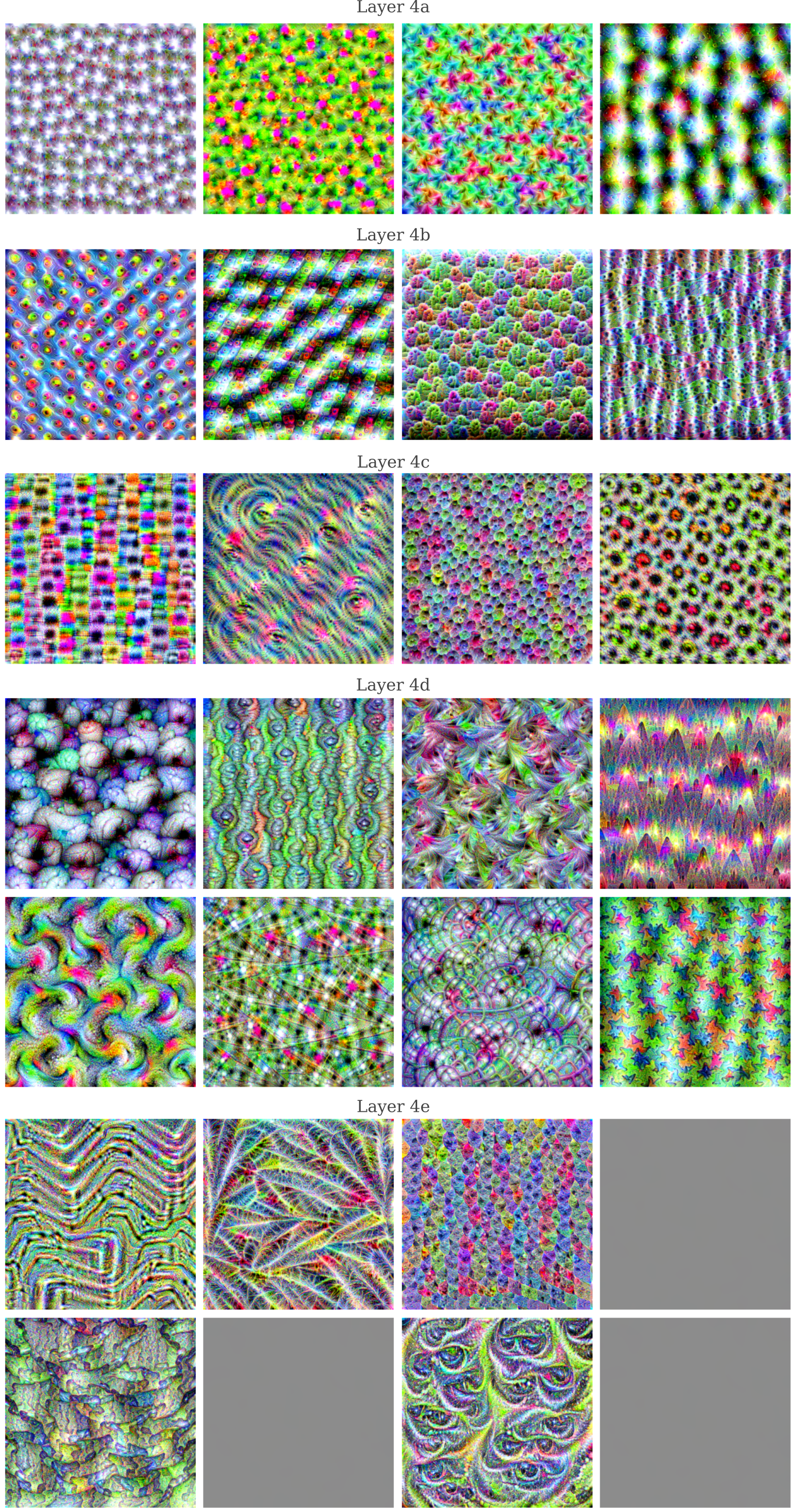
We have the following feature maps using the same optimization procedure denoted in the previous section. The starting convolutional layers are similar to what is found in the InceptionV3 model: solid colors and simple patterns are found.

Relatively early, more complex patterns are formed and objects such as small parts on animal faces are observed.

For the last two mixed convolutional layers,

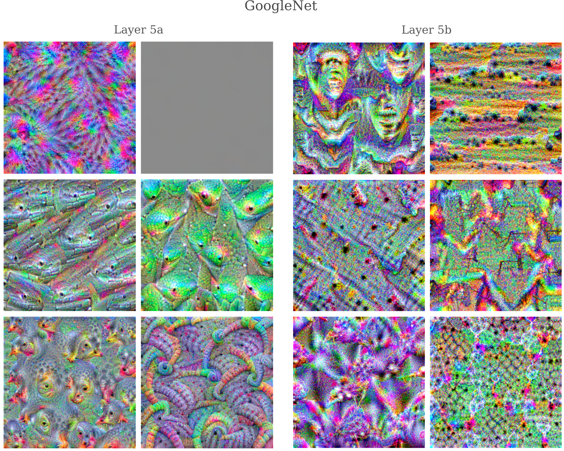
Compared to the final two layers of InceptionV3, we find that indeed there are more coherent images produced by GoogleNet (particularly for features of layer 5a, which contains recognizable snakes and bird faces).

Mapping ResNet Features

Both GoogleNet and InceptionV3 architectures are based on variants of what was originally called the Inception module, where multiple convolutional layers are applied in parallel. It may be wondered how much this architecture contributes to the feature maps that we have observed above: would a convolutional network without parallel layers also exhibit a similar tendancy for early layers to respond to simple patterns, middle layers to be activated by objects, and late layers activated by many objects together?

Another well-performing network for ImageNet-based tasks is ResNet, an architecture named after its judicious use of residual connections. These connections consist of a normal convolutional layer added elementwise to the convolutional operation input

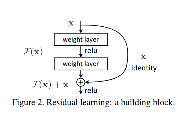
The intuition behind this architecture is that each convolutional layer learns some function $F(x)$ that is ‘referenced’ to the original input $x$, meaning that $F(x)$ is not the sole source of information for the next layer as it normally is, but instead the original information in the input $x$ is retained somewhat through addition.

The original ResNet paper published a variety of closely related architectures,

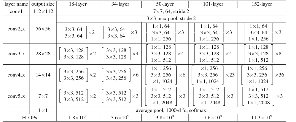
where each of the sub-modules contain residual connections. For the 50-layer version of ResNet, 8 of the first 16 features at the final layer of each module are shown below.

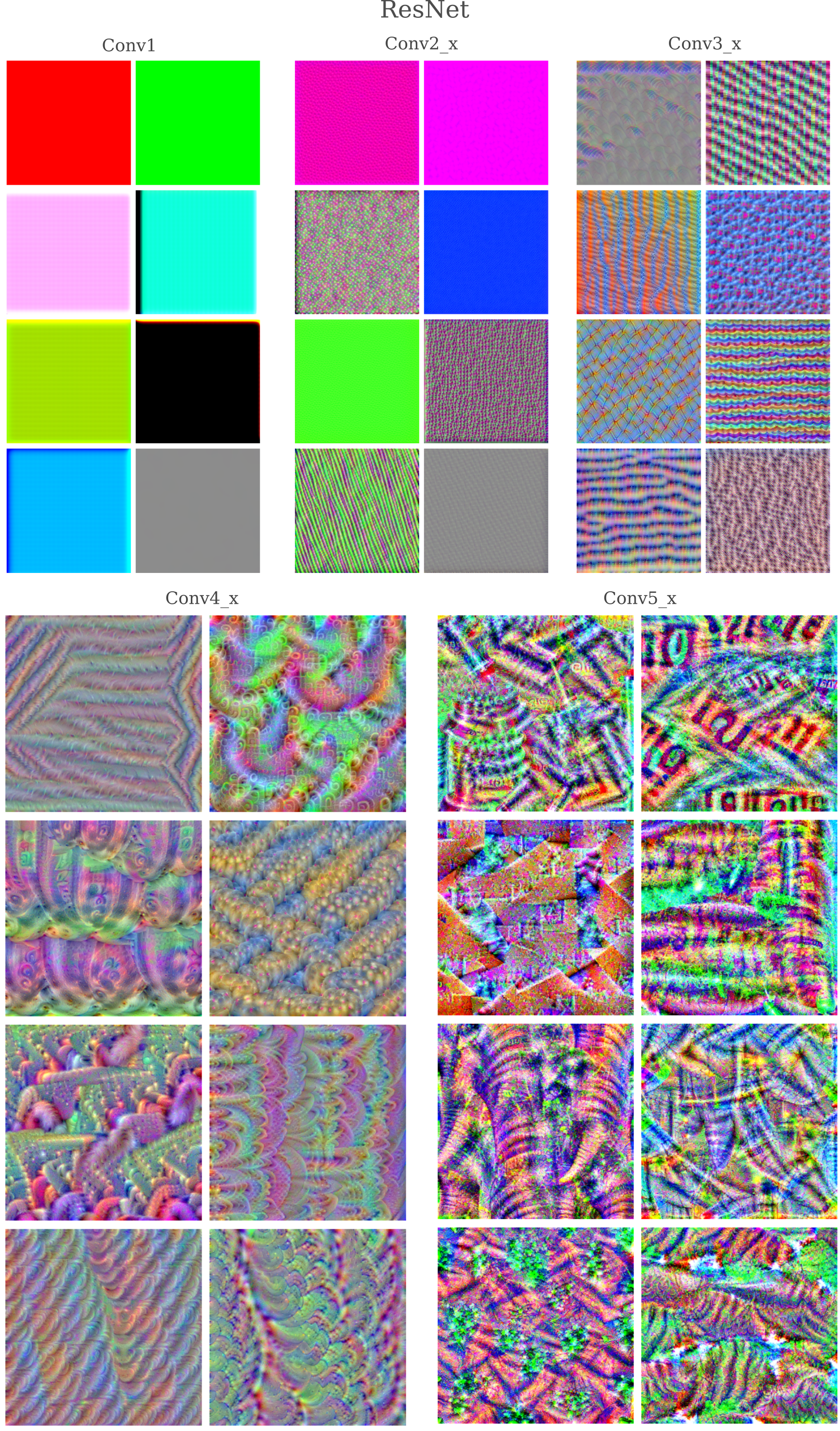
Upon examination, we see the same general features as for GoogleNet and InceptionV3: a color filter in the first convolutional layer followed by simple patterns that become more complex shapes and recognizable parts of animals in later layers. Note too that just as for both other models, features in the final layer appear to contain objects and colors that are rather jumbled together and are less coherent than in prior layers.

Layer and Neuron Interactions

Observing the images that result from gradient descent on noise gives some coherent and sometimes quite interesting feature maps. One may next wonder how all these maps work together to produce an appropriate classification label during forward propegation, or else how they can work together to generate an input representative of a certain target output category.

A first step to understanding how neurons work together has already been shown, where different neurons of one feature have been shown to be somewhat coordinated with respect to the image that results from optimizing their activations simultaneously. What about multiple neurons or even features, how do they interact in the context of generating an input image?

We therefore seek an input $a’$ that maximizes multiple multiple layers $l_1, l_2, …, l_n$, which can be equated to maximizing a single value that is the sum of the activations of those layers.

\[a' = \underset{a}{\mathrm{arg \; max}} \; \sum_{i=1}^{n} z^{l_i}(a, \theta)\]

For only two features in separate layers $l$ and $k$, the loss may be found by finding the sum of the $L_1$ distances between each layer’s activation and some large constant $C$, and therefore the gradient used to find an approximation of the target input $a’$ is

\[g = \nabla_a (C - z^{l}(a, \theta) + C - z^{k}(a, \theta))\]

It could be wondered if it would not be better to separate the gradients for each layer and then add them together during the gradient descent step

\[a_{k+1} = a_k - \epsilon * g\]

in order to ensure that both features are maximized (and not only one of these). In practical terms, the automatic differentiation engine in Pytorch gives nearly identical outputs for these two methods, so for simplicity the addition is performed before the gradient descent step. The following method implements the above equation for two features focus and focus2 that exist in layers output and output2

def double_layer_gradient(model, input_tensor, desired_output, index):
	...
	input_tensor.requires_grad = True
	output = model(input_tensor).to(device)
	output2 = newmodel2(input_tensor).to(device)

	focus = output[0][index][:][:]
	focus2 = output2[0][index][:][:]

	target = torch.ones(focus.shape).to(device)*200
	target2 = torch.ones(focus2.shape).to(device)*200

	output = model(input_tensor)
	loss = torch.sum(torch.abs(output))
	loss = (torch.sum(target - focus) + torch.sum(target2 - focus2)
	loss.backward() # back-propegate loss
	gradient = input_tensor.grad

	return gradient

There are a couple different ways we could specify the layers output and output2. Pytorch uses an automatic differentiation approach that requires all gradient sources to be specified as outputs prior to the start of forward propegation. One option to enforce this requirement is to have one model return multiple outputs, but for clarity the above method assumes multiple models are instantiated. For features in layers Conv2d_1z_3x3 and Conv2d_2z_3x3 of InceptionV3, this can be done as follows:

class NewModel2(nn.Module):

	def __init__(self, model):
		super().__init__()
		self.model = model

	def forward(self, x):
		# N x 3 x 299 x 299
		x = self.model.Conv2d_1a_3x3(x)
		return x
		
class NewModel(nn.Module):

	def __init__(self, model):
		super().__init__()
		self.model = model

	def forward(self, x):
		# N x 3 x 299 x 299
		x = self.model.Conv2d_1a_3x3(x)
		# N x 32 x 149 x 149
		x = self.model.Conv2d_2a_3x3(x)
		return x

and these two model classes may be called using a pretrained InceptionV4 model.

Inception3 = torch.hub.load('pytorch/vision:v0.10.0', 'inception_v3', pretrained=True).to(device)
newmodel = NewModel(Inception3)
newmodel2 = NewModel2(Inception3)

We can now observe how two features from arbitrary layers interact. For feature 199 of layer Mixed 6a combined with feature 201 of layer Mixed 6b, we have

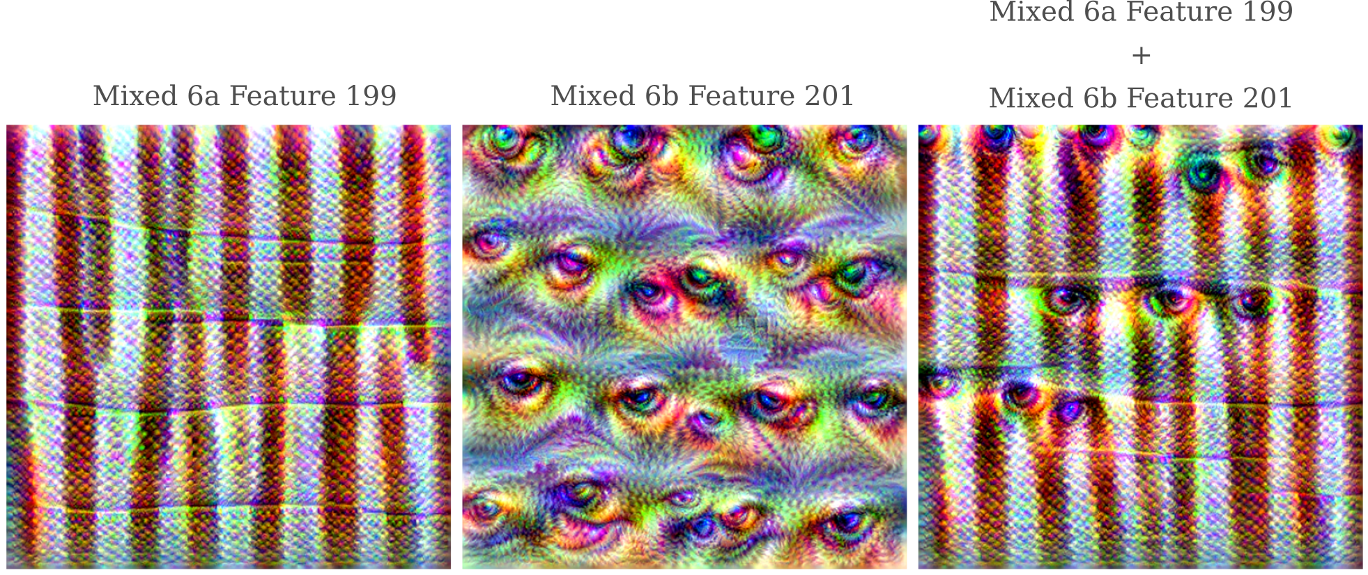
Observe how the combination is far from linear: in certain areas of the image, eyes from layer Mixed 6b are found, wheras in other areas they are completely absent.

For a detailed look at the optimization of many features at once when the original input $a_0$ is a natural image, see part II.