Feature Visualization II: Deep Dream

Introduction with Feature Optimization

In Part I, deep learning model convolutional features were investigated by constructing an input that resulted in the highest total activation in that feature, starting with random noise. But the training dataset for the models used (ImageNet) does not contain any images that resemble pure noise, making the initial input $a_0$ somewhat artificial. What happens if we start with a real image for $a_0$ rather than noise and modify that image using gradient descent?

To recap, an input $a$ may be modified via gradient descent where the gradient at step $n$, denoted $g_n$, is some loss function of the output $J(O)$ on the input $a_n$, given model parameters $\theta$,

\[g_n = \nabla_a J(O(a_n, \theta))\]

On the page referenced above, we optimized the output activation of interest $\widehat y_n$ by assigning the loss function of the output layer $J(O)$ to be the difference $J(O(a, \theta)) = C - \widehat y_n$ where $C$ is some large constant and the initial input $a_0$ is a scaled normal distribution. But gradient descent alone was not found to be very effective in producing recognizable images on $a_0$, so two additional Bayesian priors were added: smoothness (ie pixel cross-correlation) via Gaussian convolution $\mathcal{N}$ and translational invariance with Octave-based jitter, here denoted $\mathscr{J}$, were employed with the gradient for input $a_n$, denoted $g_n$. The actual update procedure is

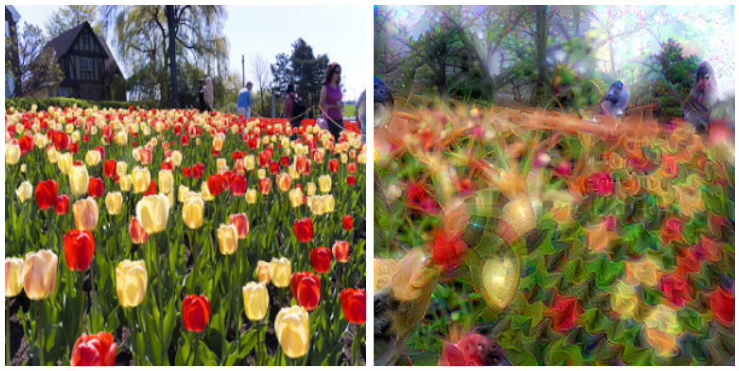
\[a_{n+1} =\mathscr{J} \left( \mathcal{N}(a_n + \epsilon g_n) \right)\]

Now we will investigate a similar update, but using octaves without jitter (denoted $\mathscr{O}$). This is done by increasing the image resolution and feeding the entire image into the model, rather than a randomly cropped version.

\[a_{n+1} =\mathscr{O} \left( \mathcal{N}(a_n + \epsilon g_n) \right)\]

A three-octave approach was found to result in clear images.

# original image size: 299x299
single_input = directed_octave(single_input, target_output, 100, [0.5, 0.4], [2.4, 0.8], 0, index, crop=False)

single_input = torchvision.transforms.Resize([380, 380])(single_input)
single_input = directed_octave(single_input, target_output, 100, [0.4, 0.3], [1.5, 0.4], 330, index, crop=False)

single_input = torchvision.transforms.Resize([460, 460])(single_input)
single_input = directed_octave(single_input, target_output, 100, [0.3, 0.2], [1.1, 0.3], 375, index, crop=False)

We will start by optimizing one or two features at a time. To do this, we want to increase the activation of each neuron in that feature using gradient descent. One way to accomplish this is to assign the loss function $J(O(a, \theta))$ to be the sum of the difference between each neuron’s activation in the feature of interest, as a tensor denoted $z^l_f$, and some large constant $C$ (denoted as a tensor as $\pmb{C}$.

\[g = \nabla_a(J(O(a; \theta))) = \nabla_a(\pmb{C} - z^l_f) \\ = \nabla_a \left(\sum_m \sum_n C - z^l_{f, m, n} \right) \\\]

As was done for feature visualization, computation of the gradient can be implemented with $C=200$ as follows:

def layer_gradient(model, input_tensor, desired_output, index):
	...
	input_tensor.requires_grad = True
	output = model(input_tensor).to(device)
	focus = output[0][index][:][:] # optimize the feature of interest
	target = torch.ones(focus.shape).to(device)*200
	loss = torch.sum(target - focus)
	loss.backward()
	gradient = input_tensor.grad
	return gradient

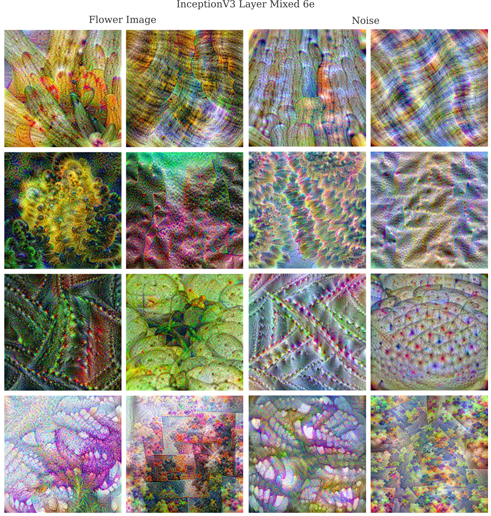
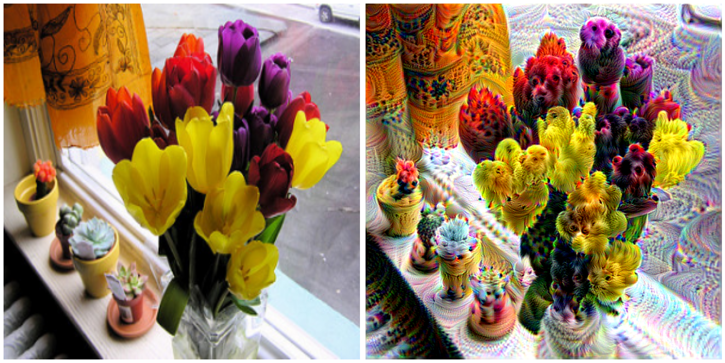
For this procedure applied to 8 features from layer Mixed 6e in InceptionV3 where the original input $a_0$ is an image of flowers, we have

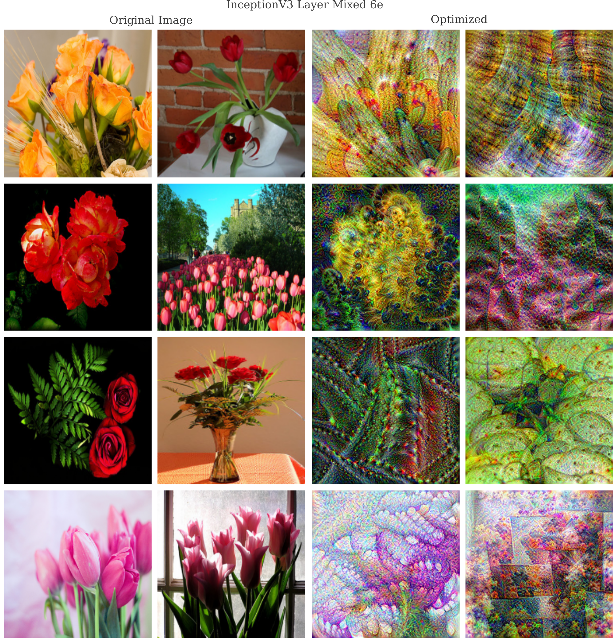
It may be wondered if there is any meaningful difference between this procedure and feature visualization in which $a_0$ is scaled Gaussian noise. Are there noticable differences after gradient descent when certain features are optimized with noise or real images as the original inputs? We can investigate this question by comparing the images generated above to those using the same optimization method but starting from the following scaled normal distribution

single_input = (torch.rand(1, 3, 299, 299))/10 + 0.5 # scaled distribution initialization

and it is apparent that the input does influence the optimized image noticably for a number of features in Layer Mixed 6e.

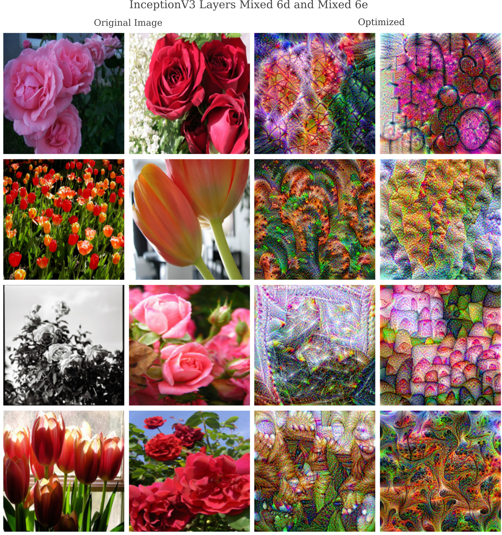
One can also modify the input $a$ such that multiple layers are maximally activated: here we have features from layers ‘Mixed 6d’ and ‘Mixed 6e’ jointly optimized by assigning the total loss to be the sum of the loss of each feature, again using a collection of flowers $a_0$.

Layer Optimization

What happens if the input image were optimized without enforcing smoothness, or in other words omitting the Gaussian convolutional step during gradient descent? We can implement gradient descent using octaves but without Gaussian convolution,

\[a_{n+1} =\mathscr{O} (a_n + \epsilon g_n)\]

as follows:

def octave(single_input, target_output, iterations, learning_rates, sigmas, index):
	...
	start_lr, end_lr = learning_rates
	start_sigma, end_sigma = sigmas
	for i in range(iterations):
		single_input = single_input.detach() # remove the gradient for the input (if present)
		input_grad = layer_gradient(newmodel, input, target_output, index) # compute input gradient
		single_input -= (start_lr*(iterations-i)/iterations + end_lr*i/iterations)* input_grad # gradient descent step
	return single_input

The other change we will make is to optimize the activations of an entire layer $\pmb z$ rather than only one or two features. One way to do this is to optimize the sum $z^l$ of the activations of layer $\pmb z^l$

\[z^l = \sum_f \sum_m \sum_n \pmb{z}^l_{f, m, n}\]

which is denoted as the sum of the tensor [:, :, :] of layer $l$. The optimization of all the features in a layer may be implemented as follows:

def layer_gradient(model, input_tensor, desired_output, index):
	...
	input_tensor.requires_grad = True
	output = model(input_tensor).to(device)
	focus = output[0][:][:][:] # optimize all features of an input
	target = torch.ones(focus.shape).to(device)*200
	loss = torch.sum(target - focus)
	loss.backward()
	gradient = input_tensor.grad
	return gradient

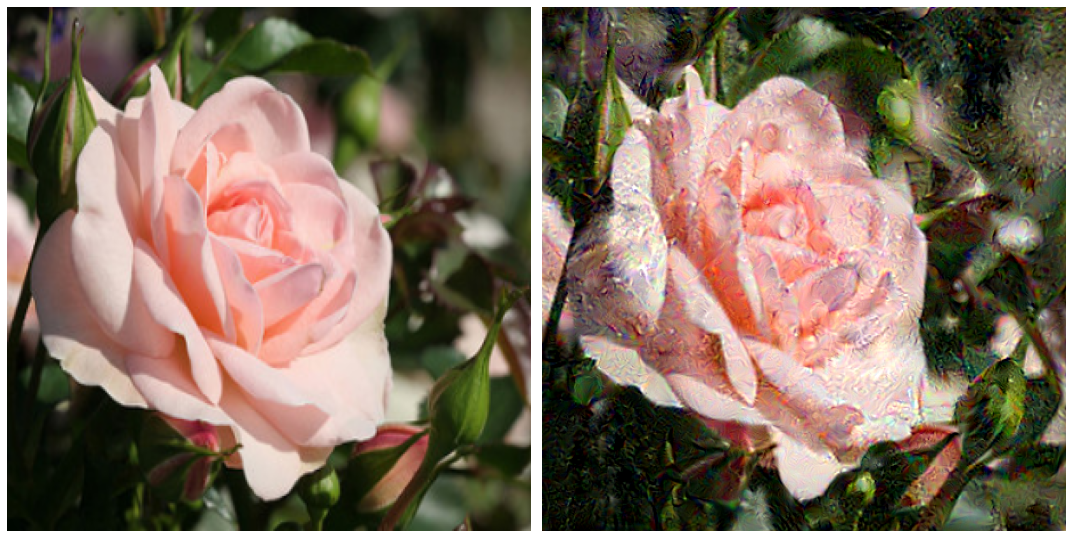
Using InceptionV3 as our model and applying gradient descent in 3 octaves to an input of flowers, when optimizing layer Mixed 6b we have

Other models yield similar results, for example optimizing layer 3 of ResNet gives

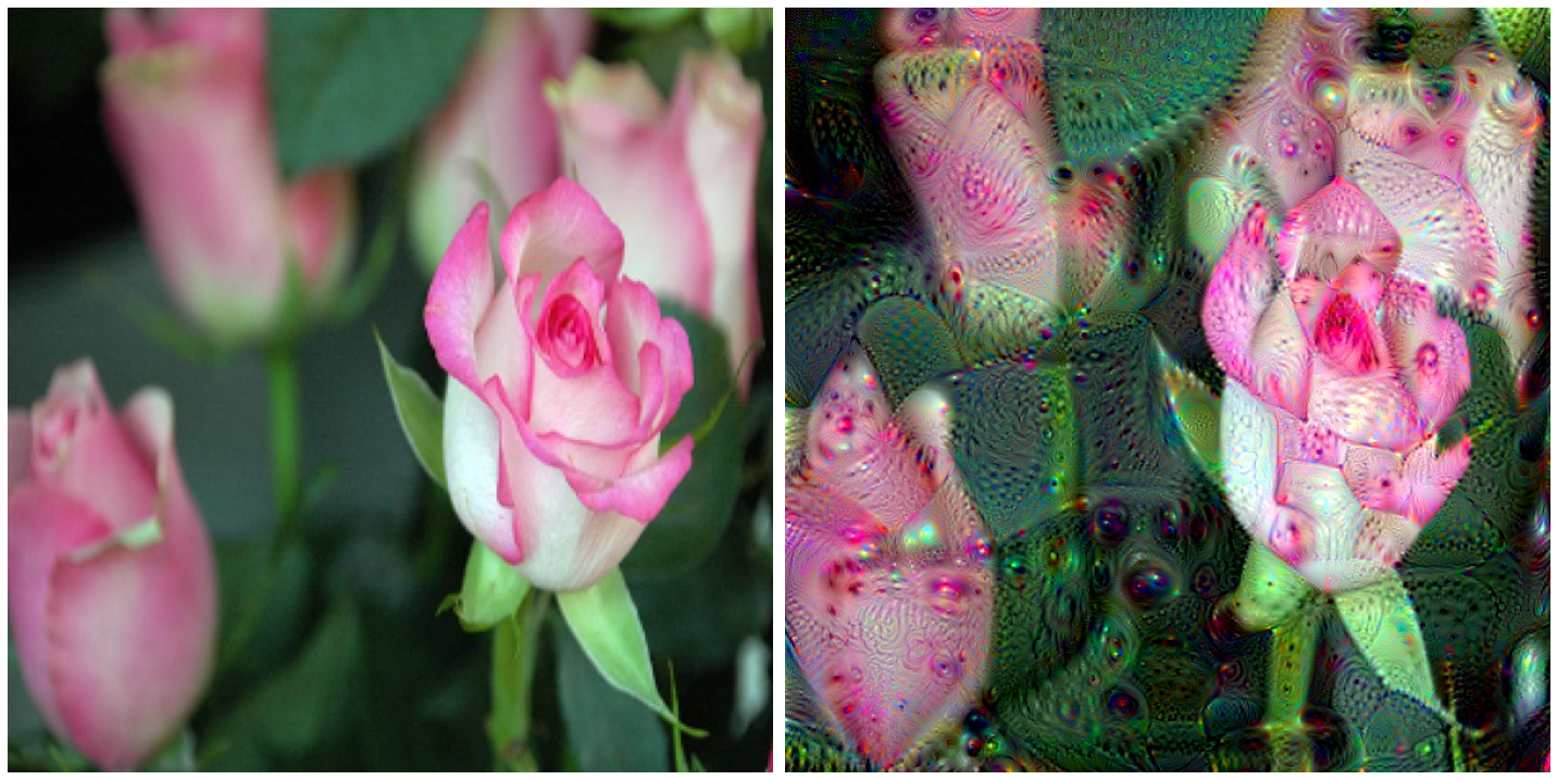
Image Resolution Flexibility

One interesting attribute of convolutional layers is thay they may be applied to inputs of arbitrary dimension.

As for feature maps, we can apply the gradient descent procedure on inputs of abitrary resolution because each layer is convolutional, meaning that only the weights and biases of kernals are specified such that any size of image may be used as input $a$ without having to change the model parameters $\theta$. Note that this is only true if all layers up to the final are convolutional: as soon as one desires use of a fully connected architecture, it is usually necessary to use a fixed input size. Right click for images at full resolution.

Note, however, that there is a clear limit to this procedure: although the input image resolution may be increased without bound, the convolutional kernals of the model in question (here InceptionV3) during training were learned only for the resolution that training inputs existed at. This is why an increase in resolution yields smaller details introduced relative to the whole image, as the changes during gradient descent are made by a model that learned to expect images of a lower resolution.

How Deep Dream makes Coherent Images

It may be wondered how deep dream makes any kind of recognizable image at all. For input image generation, we saw that gradient descent on an initial input of random noise did not yield any recognizable images, and this was for only one neuron or feature at a time rather than for many features as we have here. It was only after the addition of a smoothness Bayesian prior that gradient descent was able to begin to produce recognizable images, but smoothness is typically not added during deep dream.

Futhermore, when one considers how a convolutional layer works for image classification, it is not immediately clear how optimizing the activation of many layers together would give anything other than an incoherent jumble. This is because during feed-forward operation each feature map in a convolutional layer is expected to have a different activation corresponding to which features are found in the image one wants to classify. Activating all the feature maps is equivalent to saying that one wants an image that has all possible features, and for deeper layers with many (>= 256) features one may reasonably expect that this image will not look like much of anything at all, especially when no smoothness constraint is enforced.

After some consideration, the situation may not seem as bad as at first glance. The deep dream process begins using a natural image rather than noise, and therefore although we don’t enforce statistical characteristics of natural images during gradient descent we have enforced them at the beginning of gradient descent.

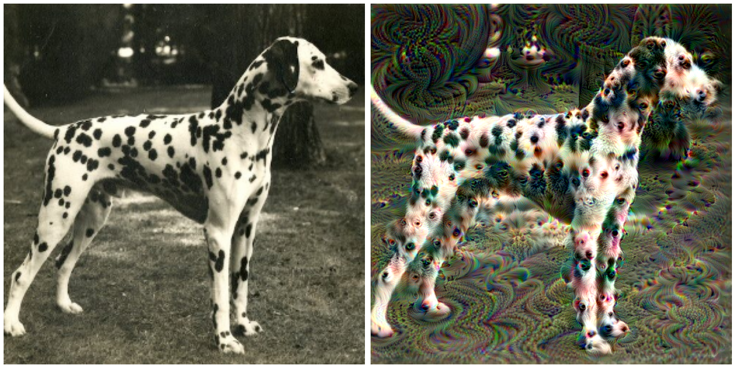
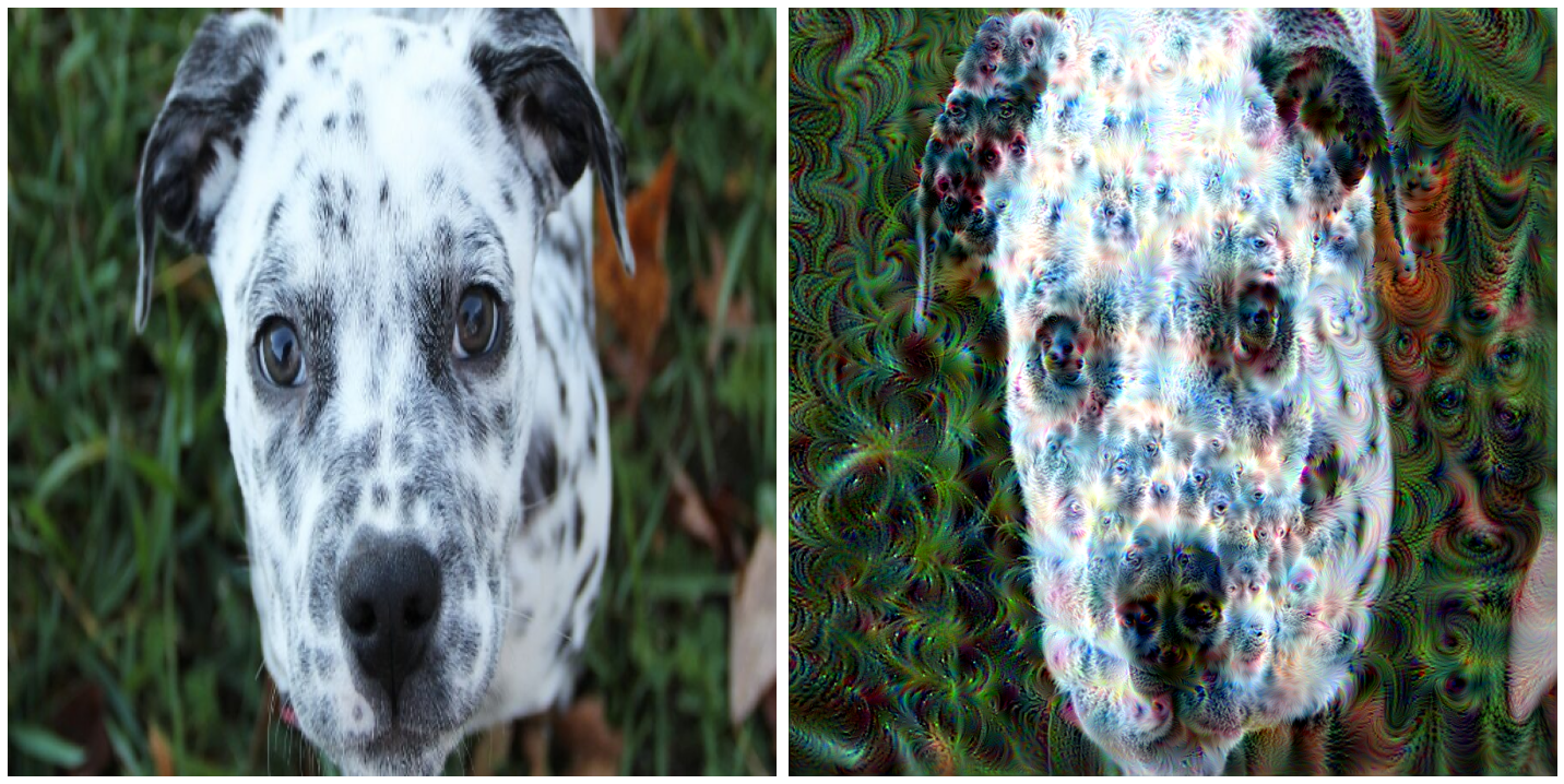
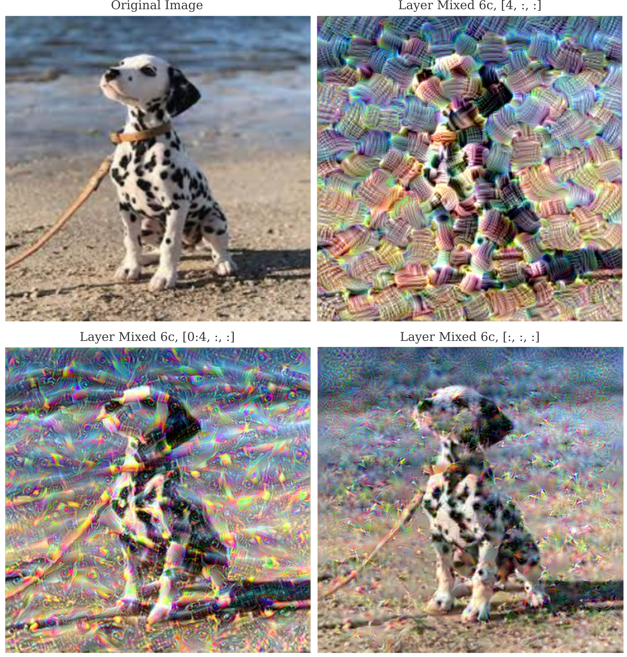
To see why optimizing the activation of many features at once does not necessarily lead to a nonsensical image, consider the following example in which first one, then five, and then all 768 features of InceptionV3’s layer Mixed 6c are optimized. As we saw in part 1, the following maps were found to maximally activate each of the first five features of layer Mixed6c:

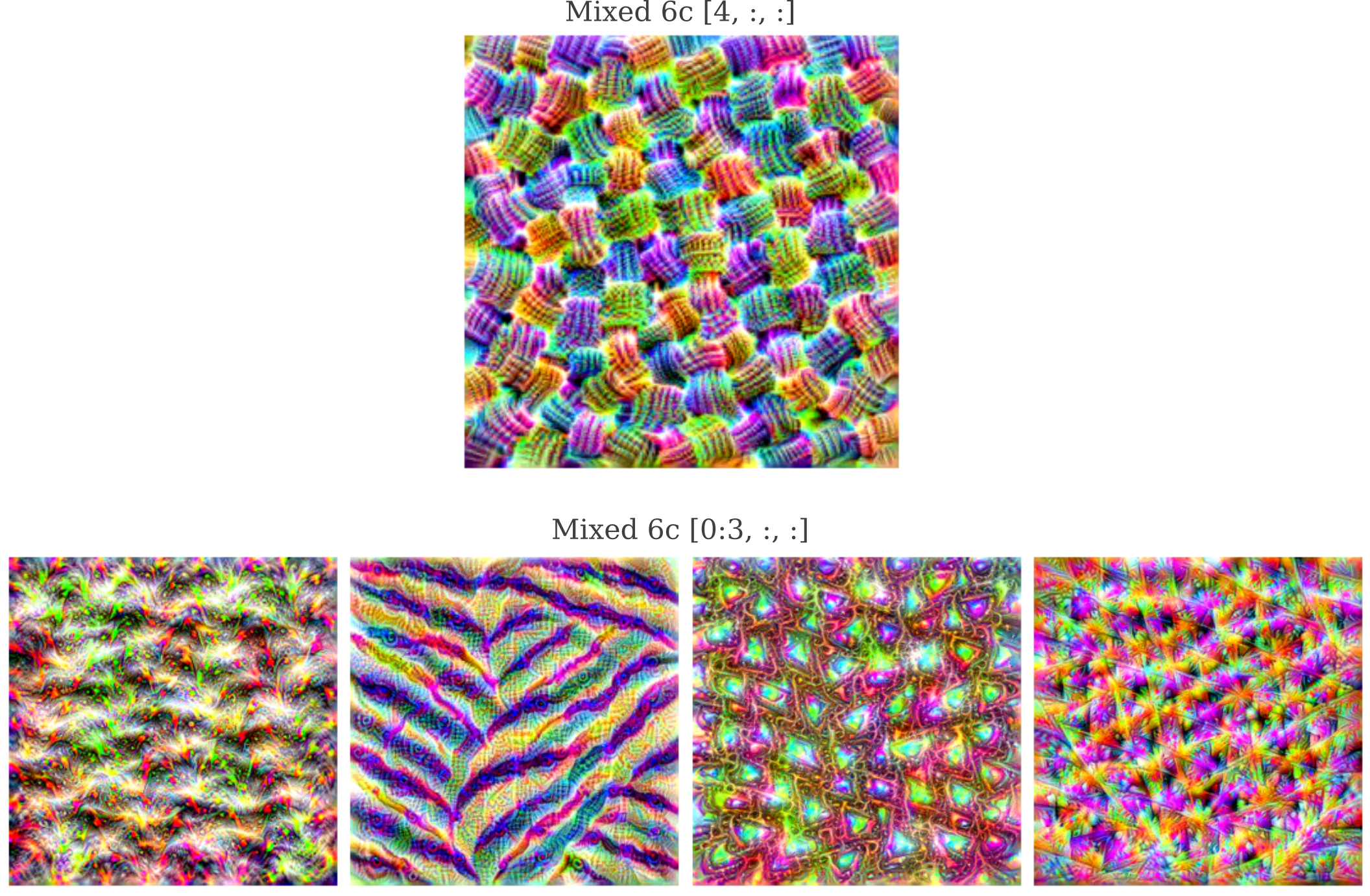
These inputs were generated from noise, but nevertheless if one particular feature were to be activated by a certain pattern, one would expect this to be the case if the starting point were not noise but instead an image of some kind. Indeed we see that is the case: observe how feature 4 gives a very similar yarn-like appearance when the starting point is a picture of a dalmation (top right below) as when it is noise (above).

On the bottom row, multiple features are optimized simultaneously. It is necessary to scale back the gradient to avoid producing very high-frequency or saturated final inputs, and we can do this by simply weighting the gradient of the entire layer by a fraction corresponding to the inverse of the number of features in that layer: ie if there are around 1000 features in a given layer, we can divide the gradient of the layer by 1000. This is because the gradient is a linear operator and is therefore additive, meaning that the gradient of an entire layer $z^l$ is equivalent to the gradient of each feature added together,

\[g = \nabla_a(J(O(a; \theta))) = \nabla_a(z^l) \\ = \nabla_a \left( \sum_f \sum_m \sum_n z^l_{f, m, n} \right) \\ = \sum_f \nabla_a \left( \sum_m \sum_n z^l_{f, m, n} \right)\]

Therefore the gradient descent update performed may be scaled by the constant $b$ while keeping the same update $\epsilon$ as was used for optimization for an individual feature. In the example above, $b=1/1000$ and

\[a_{n+1} = a_n - \epsilon * b * g_n\]

How then can we hope to make a coherent image if we are adding small gradients from nearly 1000 features? The important thing to remember is that a single image cannot possibly optimize all features at once. Consider the following simple example where we want to optimize the output of two features, where the gradient of the first feature $g_0$ for a 2x2 input $a$ is

\[g_0 = \begin{bmatrix} 1 & -1 \\ -1 & 1 \\ \end{bmatrix}\]

whereas another feature’s gradient $g_1$ is

\[g_1 = \begin{bmatrix} -1 & 1 \\ 1 & -1 \\ \end{bmatrix}\]

now as gradients are additive, the total gradient $g = g_0 + g_1$ is

\[g = \begin{bmatrix} 0 & 0 \\ 0 & 0 \\ \end{bmatrix}\]

which when applied to the original input $a$ will simply yield $a$, so clearly neither feature’s activations are optimized.

What this means is that the deep dream procedure gives what can be thought of as a kind of ‘average’ across all features in the layers of interest. As each layer must pass the entirety of the necessary information from the input to the output for accurate classification, one can expect for the dream procedure to produce shapes that are most common in the training dataset used, provided the features recognizing these images may be optimized from the input. This is why deep dream performed on sufficiently deep layers generally introduces animal objects, whereas a dataset trained on landscapes generates images of landscapes and buildings during deep dream (reference).

We can observe this inability to optimize all features during the dream process. Observe how the average feature activation does not change for many features even after 3 octaves of deep dream:

Omitting smoothness has a notable justification: the starting input is a natural image that contains the smoothness and other statistical features of other natural images, so as long as we do not modify this image too much then we would expect to end with something that resembles a natural image. But if we try to optimize the activation of some output category without smoothness, say to make an image of a ‘Junco, Snowbird’, we find that only noise has been added to the original image.

This suggests that simply starting with a natural image is not the reason why smoothness can be omitted from gradient descent during deep dream. Instead, observe how the average feature activation increased smoothly in the last video, and compare that to the discontinuous increases seen in the first video on this page (in which gradient descent without smoothness is used to optimize an output category). As the loss function in both cases is a measure of the values displayed at each time step of those videos, it is apparent that the output of a layer is continous with respect to the input, but the output of the final layer is not.

Discontinuities in the output of the final layer with respect to the input are to be expected for most classification models of sufficient power to approximate a one-to-one function (see this link for the reason why this is) but it appears that internal layers are not discontinuous with respect to the input. Exactly why this is the case is currently unclear.

Enhancements with Dreams

In the previous section it was observed that not all features of the layer of interest were capable of increasing their mean activation during deep dream. Do certain features tend to exhibit an increase in activation, leading to a similar change in the input image for all starting images or does the image generated (and therefore the features that are activated) depend on the original input? In other words, if the dream procedure tends to generate an image that is representative of the more common examples in the dataset used to train a network, what influence does the original input image have? In the original deep dream article, it was observed that the dream procedure tends to amplify objects that the model’s layer of interest ‘sees’ in original images. It remains to be seen what influence the input has on a dream, or whether the same objects tend to be amplified no matter what input is given.

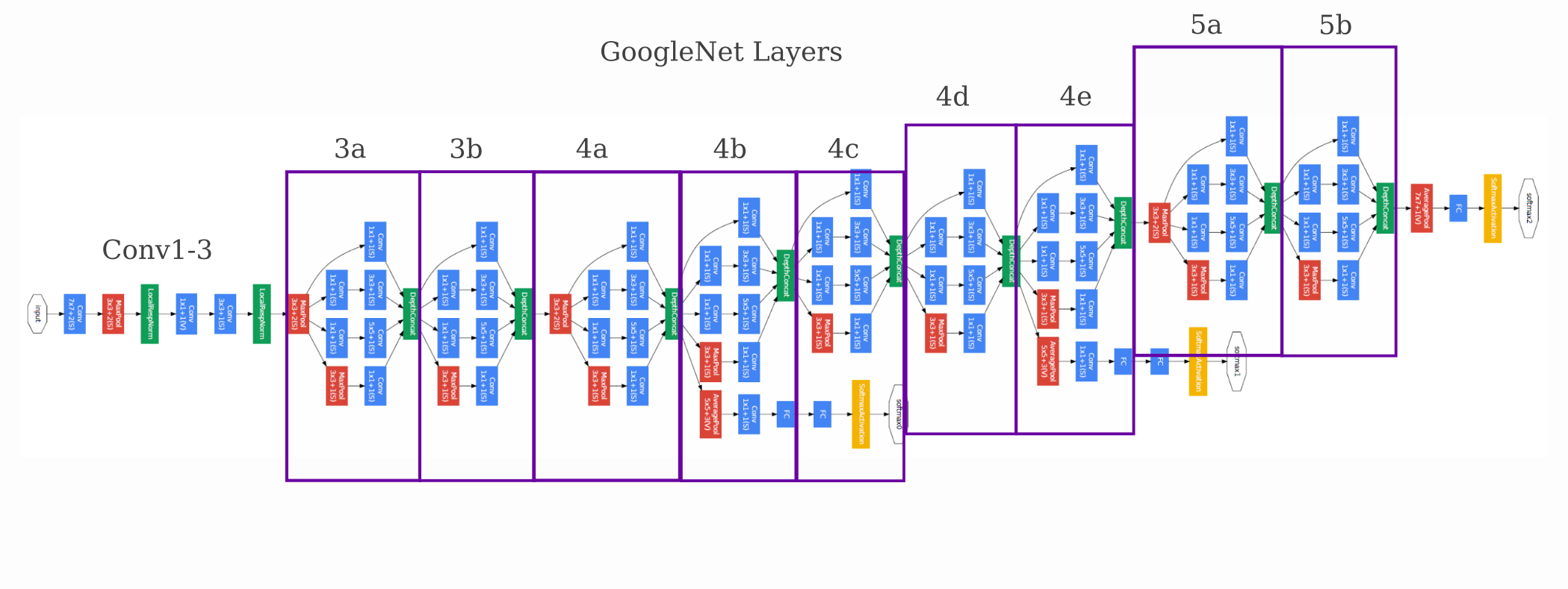
We will use GoogleNet as the model for this section. For reference, this model’s architecture is as follows:

On this page it was observed that a gradient descent on the input was capable of producing images that were confidently predicted to be of one output category. To test whether or not deep dream enhances characteristics of those categories or chooses new ones, these generated representative images will be used as initial inputs $a_0$. We apply the 3-octave gradient descent without smoothness or positional jitter, meaning the update is

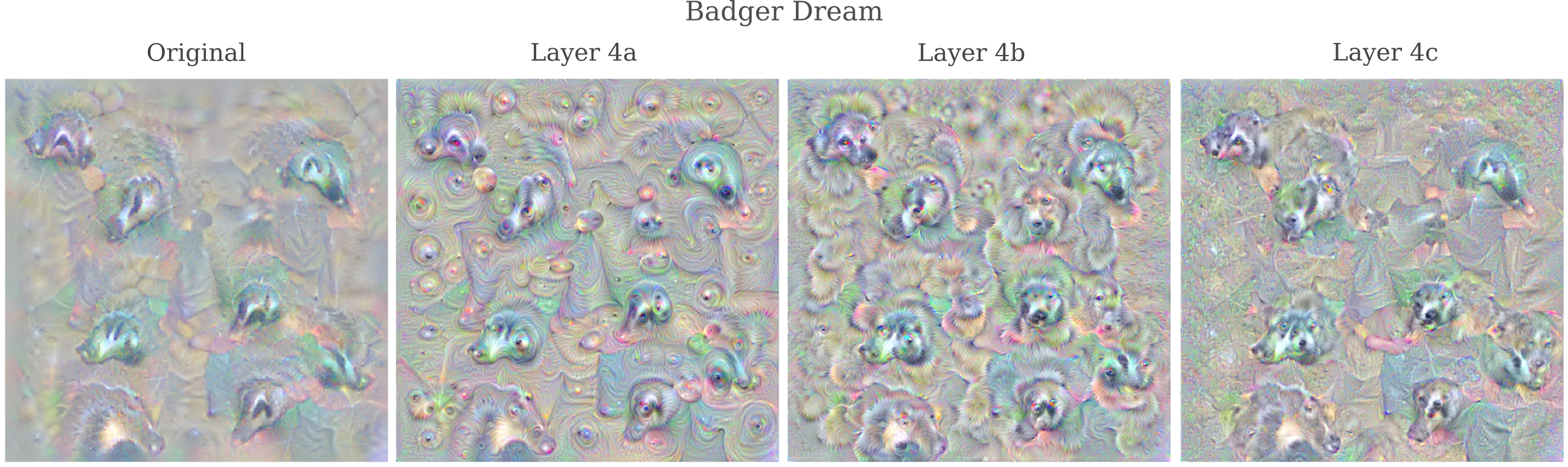
\[a_{n+1} = a_n + \epsilon * g_n\]

Optimizing layer 4c leads to an increase in the resolution on most representative ImageNet categories, for example on this image for ‘Stoplight’

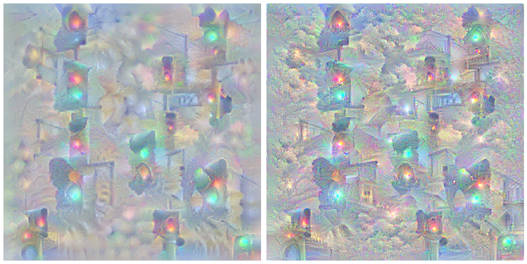
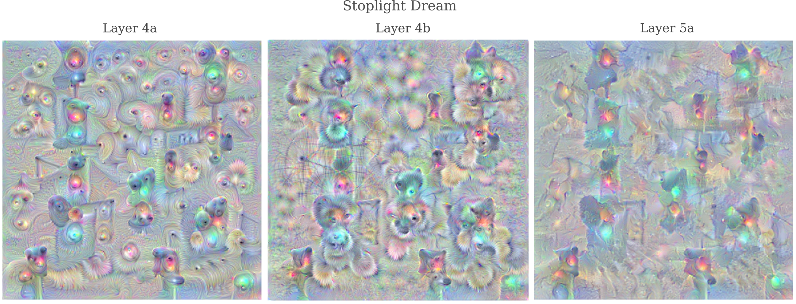
For some layers it is clear that certain characteristics are introduced irrespective of the original image $a_0$: layer 4a has introduced animal eyes and fur and layer 4b tends to add animal faces whereas layer 5a does not seem to have contributed much beyond some general textures. Particularly of note is that optimization of layer 4c has enhanced the city features of the original image (note the bridges, doors, clouds, and trees) and is of somewhat higher resolution.

For another non-animal $a_0$, we see a different result: optimization of layer 4c for ‘Volcano’ leads to the introduction of surprisingly high-resolution animal faces as well as clouds and other more realistic features

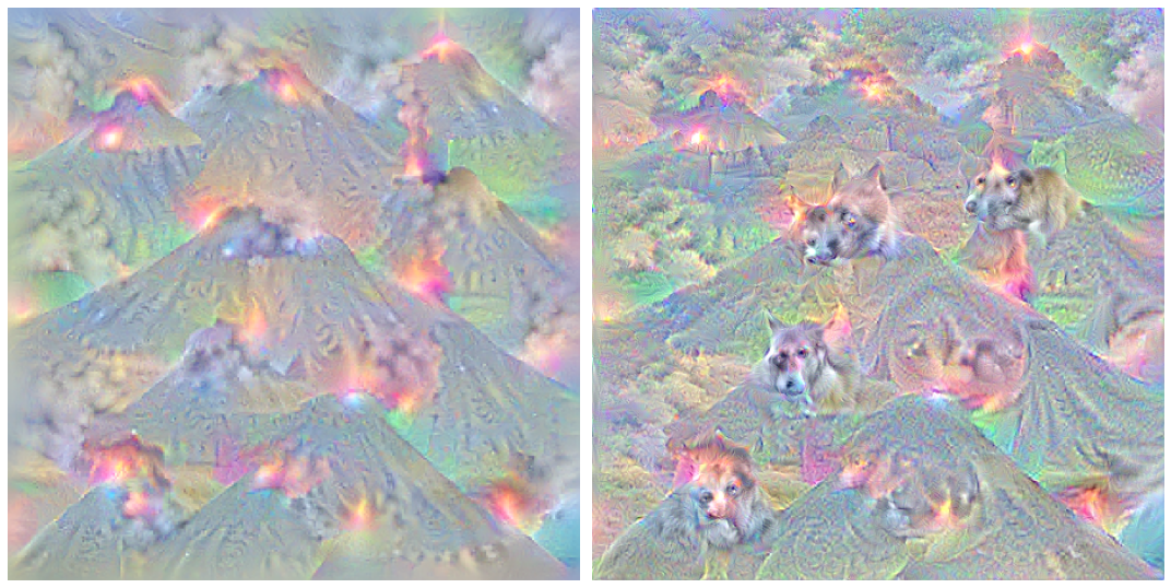
although other layers yield similar additions as for ‘Stoplight’

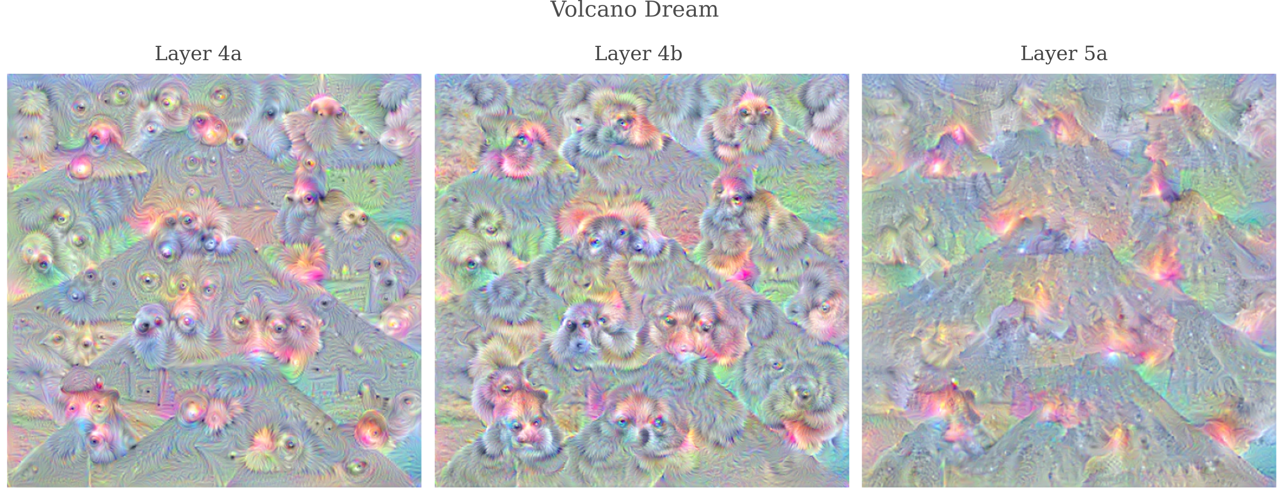
and indeed we can see that the same patterns exist for most other input images, as for example

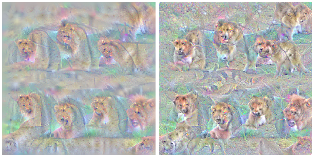
It is apparent that the final image after deep dream is of higher resolution than the initial, which is partly but not completely (see the next section) because the input generation procedure uses Gaussian blurring, but deep dream does not. This increased resolution comes at the price of some amount of precision, however, as the resulting image may not match the target category quite as well. Observe how optimizing layer 4c for an input representing ‘Lion’

and optimizing layer 4c for an input representing ‘Guinea Pig’

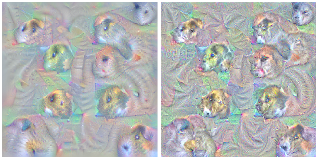
both lead to a substantial increase in resolution without high-frequency noise but do introduce certain characteristics of animals that are not the target class.

It is interesting that optimizing the activations of a hidden layer of our feed-forward network is capable of increasing the resolution of an input image. Performing gradient descent using only the output as a target nearly inevitably leads to the presence of high-frequency, incoherent structures unless some form of smoothness or local correlation is applied to the input or else the gradient.

Upon closer investigation of the representations that layer outputs are capable of forming of the input, there appears to be an explanation for why maximizing these early and middle-layer outputs would lead to an increase in resolution. For ResNet in particular, it was found that training leads to early layer kernals adopting similar weight configurations as those used to sharpen images such that the these layers learn to ‘see’ the input in more resolution than at the start of training. If these layers are activated most strongly by sharp edges, it is natural that maximizing their activations would lead to a higher-resolution image. See here for research on layer representations.

Directed Dream

As we observed in the last section, the dream procedure tends to be somewhat arbitrary with the modifications it makes to a given input: for some it introduces many new objects (usually animal faces) and for others it does not. Can the dream procedure be directed in order to introduce features that we want?

Perhaps the simplest way to direct a dream towards one object is to perform layer optimization as well as a target optimization. This can be done using gradient descent on both the layer of interest, whose gradient is $g_l$, as well as on the target with gradient $g_t$. These gradients usually have to be scaled independently, accomplished by multiplying by tensors of some constants $a$ and $b$,

\[a_{n+1} = a_n + \epsilon * (ag_l + bg_t)\]

A bit of experimentation is enough to convince on that this alone does not yield any kind of coherent image, as the same problems experienced for optimizing the gradient of the target output on this page. Namely, optimization of an output without smoothness leads to the presence of an adversarial negative with near-certainty, meaning that we cannot direct our dream by simply adding the gradient of the output class.

Instead we can enforce a small amount of smoothness using Gaussian convolution $\mathcal N$ on the modified image

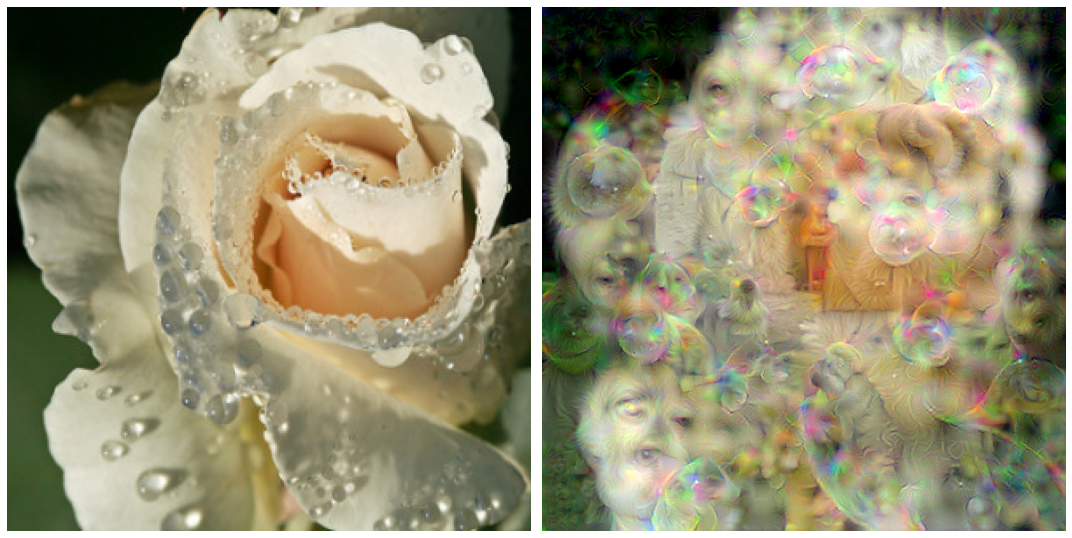
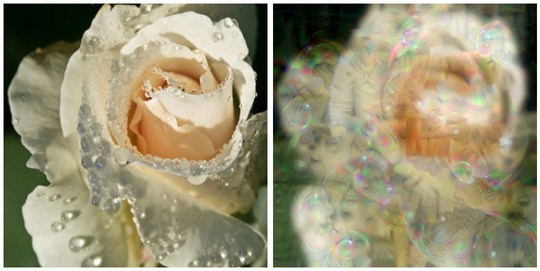
\[a_{n+1} = \mathcal{N}(a_n + \epsilon * (ag_l + bg_t))\]

where \mathcal{N} is applied only every 5 or 10 steps. Now the dream image usually contains recognizable images of the target class along with additional features that the dream might introduce. For the target class ‘Bubble’ and optimizing the activation of Layer 4c, observe how bubbles are present along with a house and some animals

Besides introducing some desired element into the dream, it is also apparent that this procedure results in higher resolution than occurs for image transfiguration where only the target class is optimized. If we apply the same smoothing procedure but with a newly scaled gradient

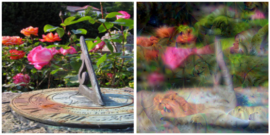
\[a_{n+1} = \mathcal{N}(a_n + \epsilon * (cg_t))\]

we find that the bubbles resulting are of somewhat lower resolution, mirroring what was observed in the last section of this page.

The increase in resolution for directed dreams relative to image transfigurations (using only the gradient of the target class) is most apparent when the target is an animal. For the target class ‘Lion’, observe how the directed dream with Layer 4c which is as follows

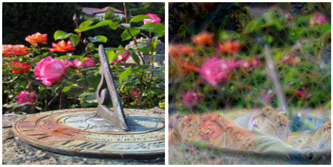
introduces lions with much higher resolution than transfiguration of the same target.

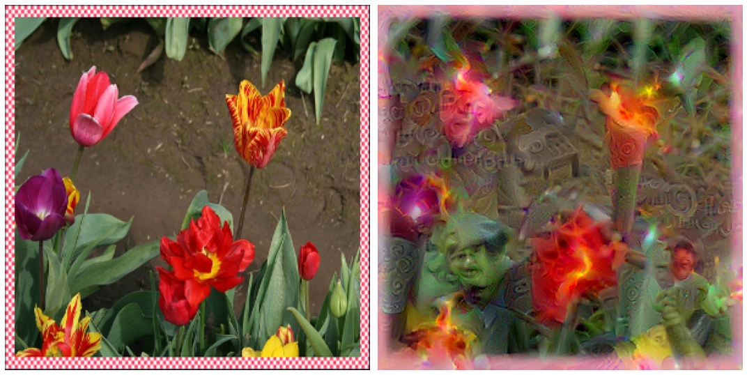
Directed dreams can introduce practically any of the 1000 ImageNet target categories, or a combination of these categories. Observe the result of the dream on Layer 4c with a target class of ‘Torch’:

or ‘Junco, Snowbird’ (note the birds on the left and right hand side of the image)