Input Representations and Depth

This page is part IV in a series on input generation, follow this link for part III.

Trivial autoencoding ability decreases with model depth

It is worth examining again what was explored in the part III: an input $a$ is fed to a model $\theta_1$ to make a target output

\[\widehat{y} = O(a, \theta_1)\]

This target output may be understood as the coordinates in a latent space ($\Bbb R^{1000}$ for ImageNet categories), and the gradient of the distance between the target output $\widehat{y}$ and the actual model’s output $y$ is minimized via gradient descent. In effect the model recieves an input and attempts to copy it using only the knowledge of the coordinates of the chosen latent space, which means that gradient descent on the input to match some latent space coordinates can accurately be described as an autoencoding of the input.

Autoencoders have long been studied as generative models. The ability of an autoencoder to capture important features of an input without gaining the ability to exactly copy the input makes these models useful for dimensional reduction as well. And it is this feature that we will explore with our classification model-based autoencoder.

Perfect representation requires that a model be able to pass all the input information to the model’s final layer, or else an identity function would not be approximated as many inputs could give one output. Are hidden layers of common deep learning classification models capable of perfect representation? The method we will use is the capability of each layer to perform an autoencoding on the input using gradient descent on a random vector as our decoder. First we pass some target image $a_t$ into a feedforward classification network of choice $\theta$ and find the activations of some given output layer $O_l$

\[\widehat y = O_l(a_t, \theta)\]

Now that the vector $\widehat y$ has been found, we want to generate an input that will approximate this vector for layer $l$. The approximation can be achieved using a variety of different metrics but here we choose $L^1$ for speed and simplicity, making the gradient of interest

\[g = \nabla_{a_n} \sum_i \lvert \widehat y - O_l(a_n, \theta) \rvert\]

The original input $a_0$ is a scaled normal distribution

\[a_0 = \mathcal {N}(0.7, 1/20)\]

and a Gaussian convolution $\mathcal{N_c}$ is applied at each gradient descent to enforce smoothness.

\[a_{n+1} = \mathcal{N_c} (a_n - \epsilon * g)\]

Thus the feed-forward network encoder may be viewed as the forward pass to the layer of interest, and the decoder as the back-propegation of the gradient combined with this specific gradient descent procedure.

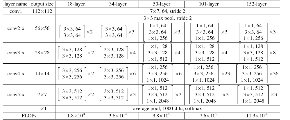
First we will investigate the ResNet family of models which have the following architecture:

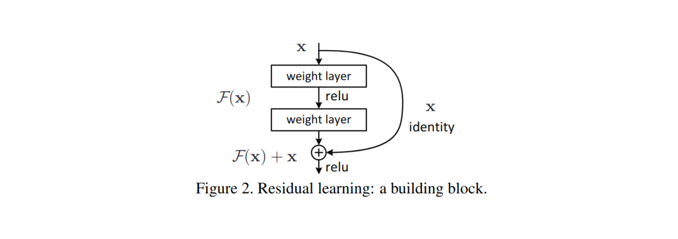
We will first focus on the ResNet 50 model. Each resnet module has a residual connection, which is formed as follows:

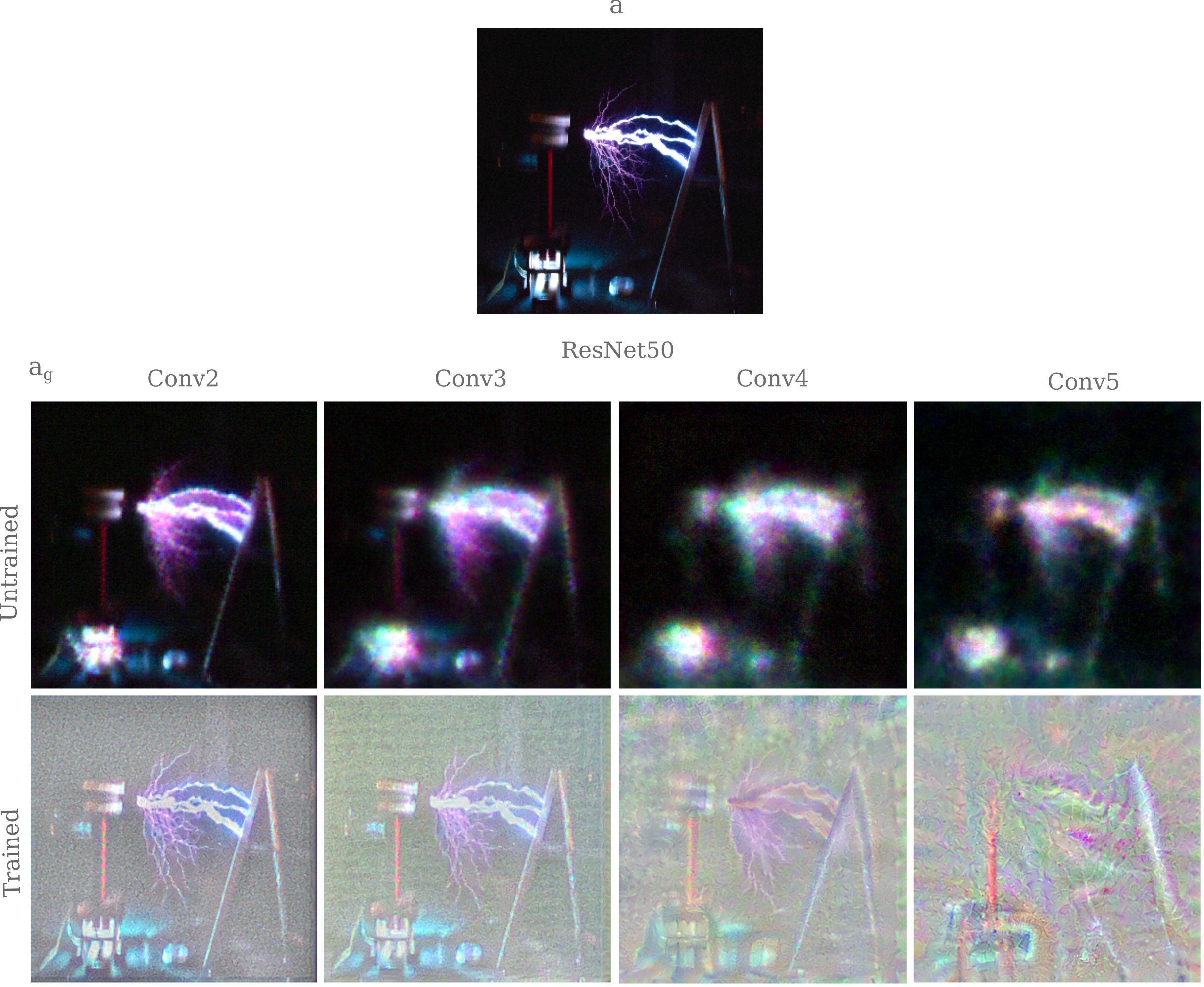
Now we will test for each layer’s ability to represent the input using our autoencoding method. We find that early layers are capable of approximately copying the input, but as depth increases this ability diminishes and instead a non-trivial representation is found.

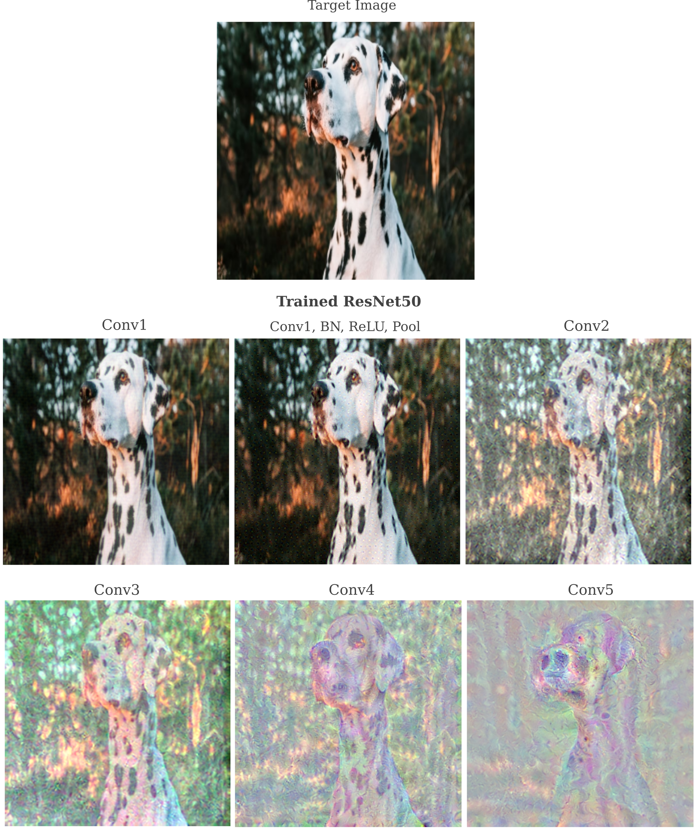
For each layer, the image formed can be viewed as a result of a trivial (ie approximate copy) and non-trivial (not an approximate copy) representation of the input. In particular, observe the pattern of spots on the dog’s fur. Trivial representations would exactly copy this patter whereas non-trivial ones would not unless this precise patter were necessary for identification (and it is not). Intuitively a trivial representation would not require any model training to approximately copy the input, as long as the decoder function is sufficiently powerful. Thus we can search for the presence of trivial representations by repeating the above procedure but for an untrained version of the same model.

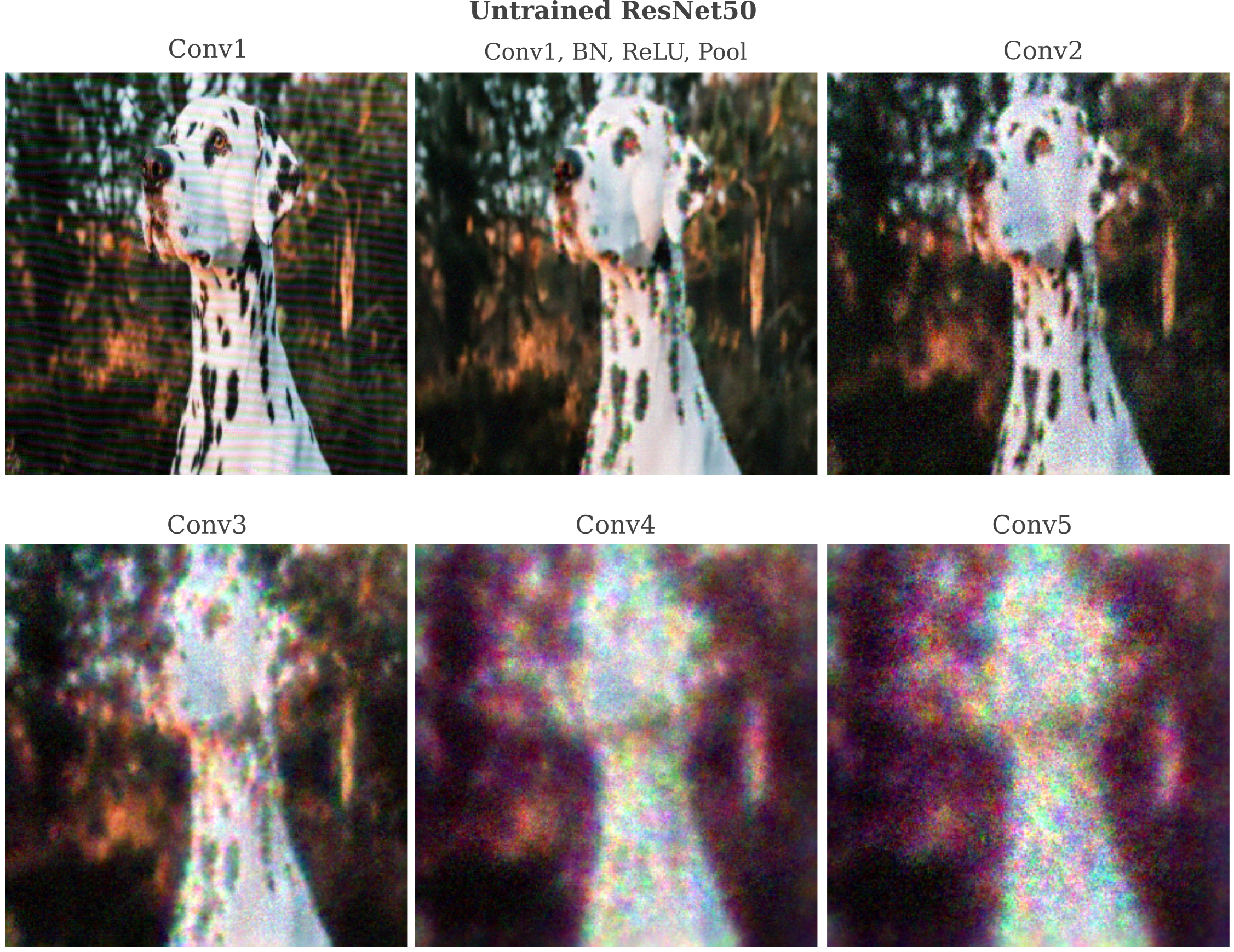
Thus we see that the untrained (and therefore necessarily trivial) representation of the input disappears in the same deeper layers that the learned (and in this case non-trivial) representation are found for trained models.

Imperfect representations are due to nonunique approximation

Why do deep layers of ResNet50 appear to be incapable of forming trivial autoencodings of an input image? Take layer Conv5 of an untrained ResNet50. This layer has more than 200,000 parameters and therefore viewing this layer as an autoencoder hidden layer $h$ would imply that it is capable of copying the input exactly, as the input has only $299*299=89401$ elements.

To understand why a late layer in an untrained deep learning model is not capable of very accurate input representation, it is helpful to consider what exactly is happening to make the input representation. First an input $a$ is introduced and a forward pass generates a tensor $y$ that is the output of a layer of interest in our model,

\[y = O(a, \theta)\]

This tensor $y$ may be thought of as containing the representation of input $a$ in the layer in question. To observe this representation, we then perform gradient descent on an initially randomized input $a_0$

\[a_{n+1} = a_n - \epsilon \nabla_{a_n} m \left( O(a_n, \theta), O(a, \theta) \right)\]

in order to find a generated input $a_g$ such that some metric $m$ between the output of our original image and this generated image is small. We employ the $L^1$ metric for gradient descent minimization, in which case the measure is

\[m = \sum_i \vert O(a_g, \theta)_i - O(a, \theta)_i \vert\]

and typically employ the $L^2$ norm of the vector difference between representations $O(a_g, \theta)$ and $O(a, \theta)$ (with a reference value) as a way of observing how effective our miminization procedure was. The $L^2$ norm between output and target output is denoted as $\vert \vert O(a_g, \theta) - O(a, \theta) \vert \vert_2$ and is defined as follows:

\[L^2 = \sqrt{\sum_i \left(O(a_g, \theta)_i - O(a, \theta)_i \right)^2}\]

One can think of each step of the representation visualization process as being composed of two parts: first a forward pass and then a gradient backpropegation step. An inability to represent an input is likely to be due to one of these two parts, and the gradient backpropegation will be considered first.

It is well known that gradients tend to scale poorly over deeper models with many layers. The underlying problem is that the process of composing many functions together makes finding an appropriate scale for the constant of gradient update $\epsilon$ very difficult between different layers, and for some instances for multiple elements within one given layer. Batch normalization was introduced to prevent this gradient scale problem, but although effective in the training of deep learning models it does not appear that batch normalization actually necessarily prevents gradient scaling issues.

However, if batch normalization is modified such that each layer is determined by variance factor $\gamma = 1$ and mean $\beta = 0$ for a layer output $y$,

\[y' = \gamma y + \beta\]

Then the gradient scale problem is averted. But the initialization process of ResNet50 does indeed set the $\gamma, \beta$ parameters to $1, 0$ respectively, meaning that there is no reason why we would expect to experience problems finding an appropriate $\epsilon$. Futhermore, general statistical measures of the gradient $\nabla_a O(a, \theta)$ are little changed when comparing deep to shallow layers, suggesting that the gradient used to update $a_n$ is not why the representation is poor.
Thuse we consider whether the forward pass is somehow the culprit of our poor representation. We can test this by observing whether the output of our generated image does indeed approximate the tensor $y$ that we attempted to approximate: if so, then the gradient descent process was successful but the forward propegation loses too much information for an accurate representation.

We can test whether the layer output $O(a, \theta)$ approximates $y$ using the $L^2$ metric above, thereby findin the measure of the ‘distance’ between these two points in the space defined by the number of parameters of the layer in question. Without knowing the specifics of the values of $\theta$ in all layers leading up to the output layer, however, it is unclear what eactly this metric means, or in other words exactly how small it should be in order to determine if an output really approximates the desired $y$.

Therefore a comparative metric is introduced: a small (ie visually nearly invisible) shift is made to the original input $a$ and the resulting $L^2$ metric between the output of the original image $y = O(a, \theta)$ and the output of this shifted image

\[m_r = ||O(a, \theta) - O(a', \theta)||_2\]

is obtained as a reference. This reference $m_r$ can then be compared to the metric obtained by comparing the original output to the output obtained by passing in the generated image $a_g$

\[m_g = ||O(a, \theta) - O(a_g, \theta)||_2\]

First we obtain $a’$ by adding a scaled random normal distribution to the original,

\[a' = a + \mathcal N (0, 1/25)\]

and then we can obtain the metrics $m_r, m_g$ in question.

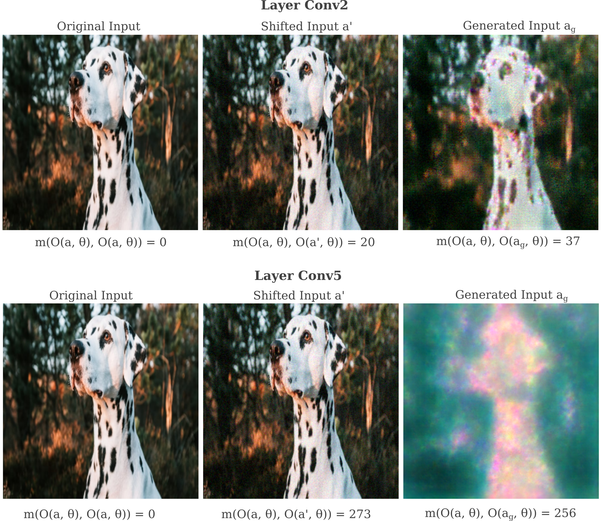
Observe that an early layer (Conv2) seems to reflect what one observes visually: the distance between $a’, a$ is smaller than the distance between $a_g, a$ as $a’$ is a slightly better approximation of $a$. On the other hand, the late layer Conv5 exhbits a smaller distance between $a_g, a$ compared to $a’, a$ which means that according to the layer in question (and assuming smoothness), there generated input $a_g$ is a better approximation of $a$ than $a’$.

It may be wondered whether this phenomenon is seen for other architectures or is specific to the ResNet50 model. Typical results for an untrained ResNet18,

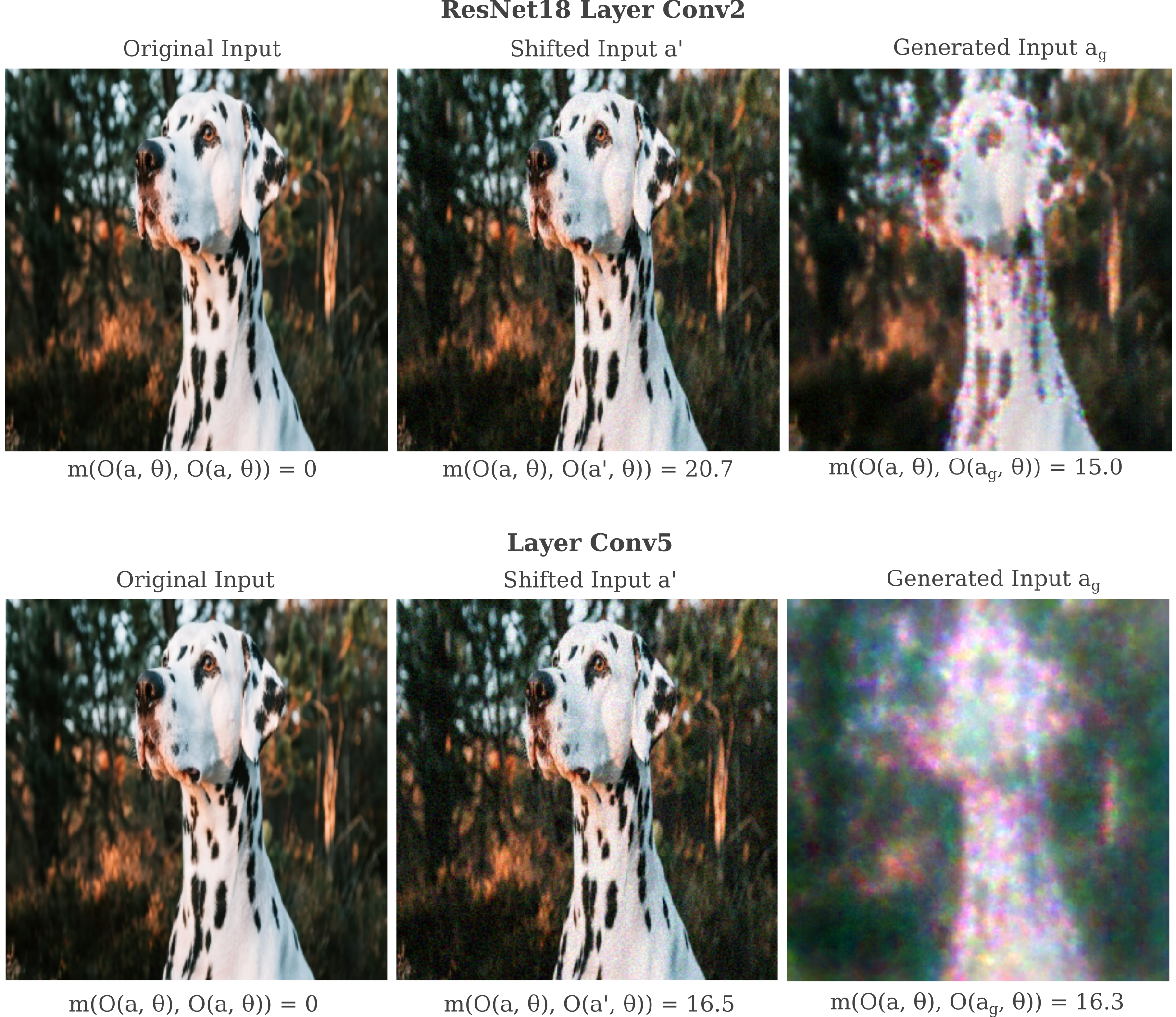
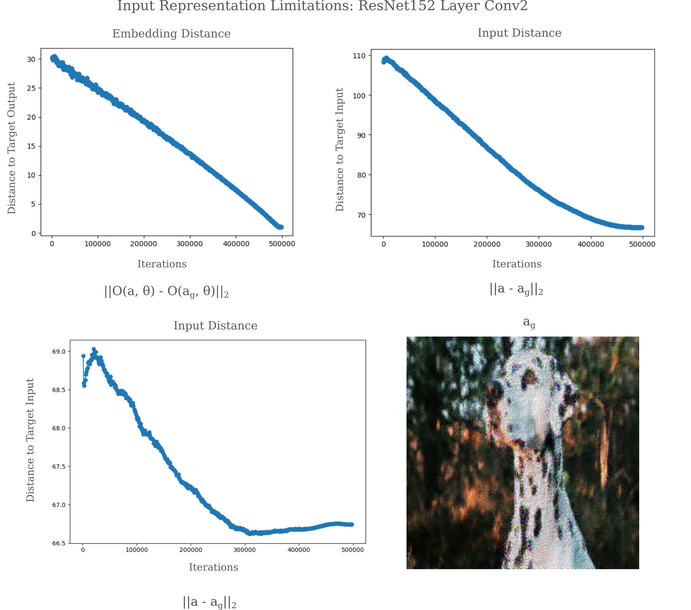
and an untrained ResNet152

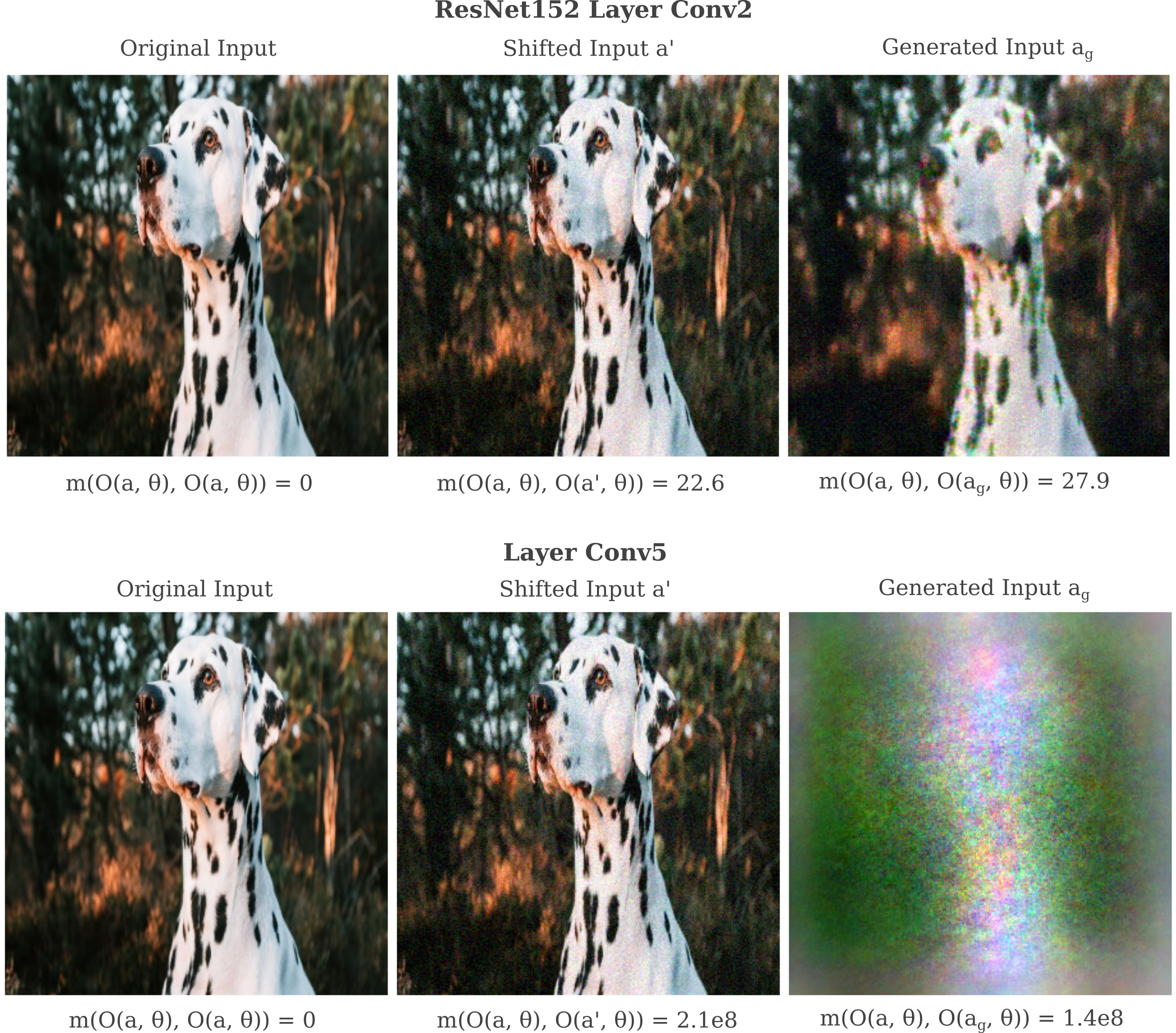
show that early and late layer representations both make good approximations (relative to a slightly shifted $a’$) of the input they attempt to approximate, even though the late layer representations are visually clearly inaccurate. Furthermore, observe how the representation becomes progressively poorer at Layer Conv5 as the model exhibits more layers. These results suggest that in general layer layers of deep learning models are incapable of accurate (trivial) untrained representation of an input not because the gradient backpropegation is necessarily inaccurate but because forward propegation results in a non-unique approximations to the input.

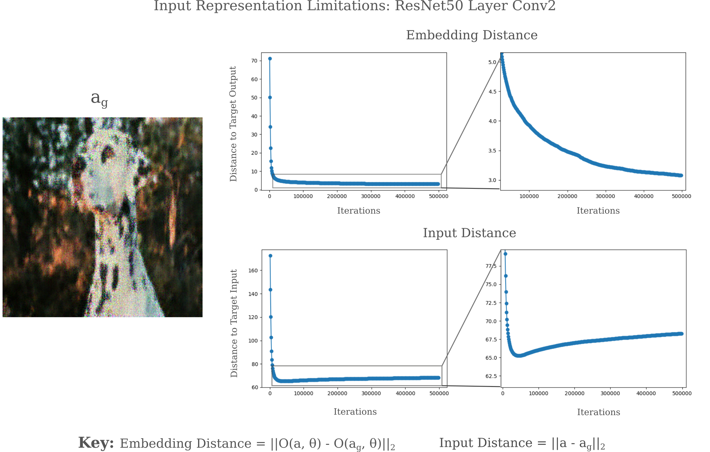
It may be wondered if a better representation method could yield a more exact input. In a later section, we will see that the $a’$ reference is atypically close to $a$ compared to other points in the neighborhood of $O(a’, \theta) - O(a, \theta)$ of $O(a, \theta)$ and thus may not be an ideal reference point. To avoid the issue of what reference in output space to use, we can instead observe the output metric $m_g$ anc compare this to the corresponding metric on the input,

\[m_i = || a_g - a ||\]

The $m_g$ metric corresponds to the representation accuracy in the output space and $m_i$ corresponds to the representation accuracy with respect to the input. Therefore we can think of $m_g$ as being a measure of the ability of the gradient descent procedure to approximate $O(a, \theta)$ while $m_i$ is a measure of the accuracy of the representation to the target input.

For even relatively shallow layers there may exist an increase in $m_i$ while $m_g$ tends towards 0. For ResNet layer Conv2, we see the latter behavior for a fixed $\epsilon$

while for ResNet152 layer Conv2, we find an asymptote of $m_i$ far from 0 while $m_g$ heads towards the origin for a variable (linearly decreasing) $\epsilon$.

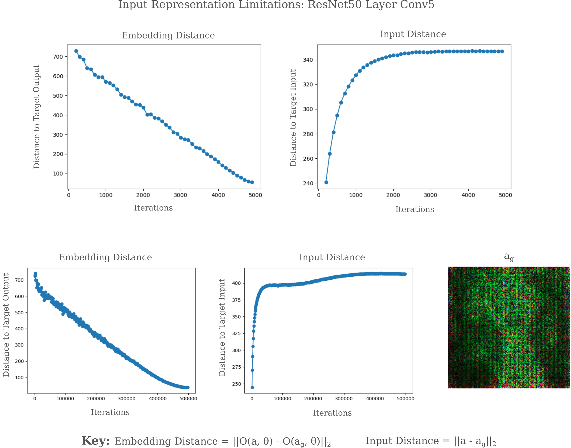
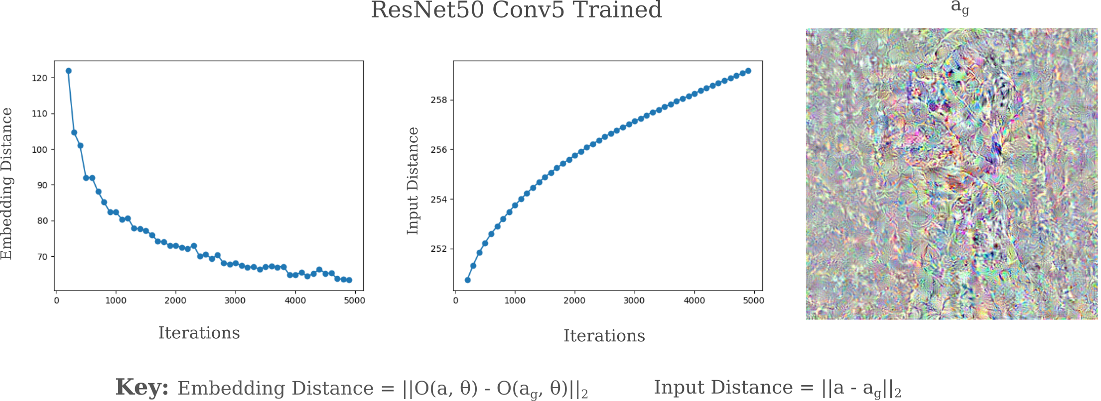
For deeper layers this effect is more pronounced: it is common for $m_i$ to increase while $m_g$ tends towards the origin for layer conv5 of resnet50.

Why depth leads to nonunique trivial representations

From the previous few sections, it was seen first that deeper layers are less able to accurately represent an input image than earlier layers for untrained models, and secondly that this poor representation is not due to a failure in the input gradient descent procedure used to visualize the representation but instead results from the layer’s inability to distinguish between very different inputs $(a, a_g)$. It remains to be explored why depth would relate to a reduction in discernment between different inputs. In this section we explore some contributing factors to this decrease in accuracy from a theoretical point of view before considering their implications to model architectures.

The deep learning vision models used on this page are based on convolutional operations. For background on what a convolution is (in the context of image processing) and why it is useful for deep learning, see this page.

What is important for this page is that these models make use of mathematical operations that are in general non-invertible. For convolutions themselves, given some input tensor $f(x, y)$, the convolution $\omega$ may be applied such that

\[\omega f(x, y) = f'(x, y)\]

does not have a unique inverse operation

\[\omega^{-1}f'(x, y) = f(x, y)\]

Specifically, a convolutional operation across an image is non-invertible with respect to the elements that are observed at any given time. Thus, generally speaking, pixels within the kernal’s dimensions may be swapped without changing the ouptut.

To see why this is, consider a simple example: a simple case of a one-dimensional convolution of shape with a uniform kernal. This kernal is

\[\omega = \frac{1}{2} \begin{bmatrix} 1 & 1 \end{bmatrix}\]

such that the convolutional operation is

\[\omega * f(x_1, y_1) = \frac{1}{2} \begin{bmatrix} 1 & 1 \end{bmatrix} * \begin{bmatrix} 2 \\ 3 \\ \end{bmatrix}\] \[\omega * f(x_2, y_2) = 1/2 (1 \cdot 2 + 1 \cdot 3) = 5/2 \\\]

Now observe that if we know the output of the convolutional operation and the kernal weights we cannot solve for the input: an infinite number of linear combinations of 2 and 3 exist that satisfy a sum of $5/2$. Invertibility may be recovered by introducing padding to the input and scanning over these known values, but in general only if the stride length is $1$.

In the more applicable case, any convolutional operation that yields a tensor of smaller total dimension ($m \mathtt{x} n$) than the input is non-invertible, as is the case for any linear operation. Operations that are commonly used in conjunction with convolutions (max or average pooling, projections, residual connections etc.) are also non-invertible.

Because of this lack of invertibility, there may be many possible inputs for any given output. As the number of non-invertible operations increases, the number of possible inputs that generate some output vector also increases exponentially. Therefore it is little wonder why there are different input $a_g, a, a’$ that all yield a similar output given that many input can be shown to give one single output even with perfect computational accuracy.

One can experimentally test whether or not non-uniqueness leads to poor representations using simple fully connected architectures. It should be noted that nearly all fully connected architectures used for classification are composed of non-invertible operations that necessarily lead to non-uniqueness in representation. Specifically, a forward pass from any fully connected layer $x$ to another that is smaller than the previous, $y$, is represented by a non-square matrix multiplication operation. Such matricies are non-invertible, an in particular the case above is expressed with a matrix $A_{m\mathrm{x}n}, m < n$ such that there are an infinite number of linear combinations of elements of $x$.

\[y = Ax \\ A^{-1}y = x\]

Whithin a specific range, there are only a finite number of linear combinations but this number increases exponentially upon matrix multiplication composition, where

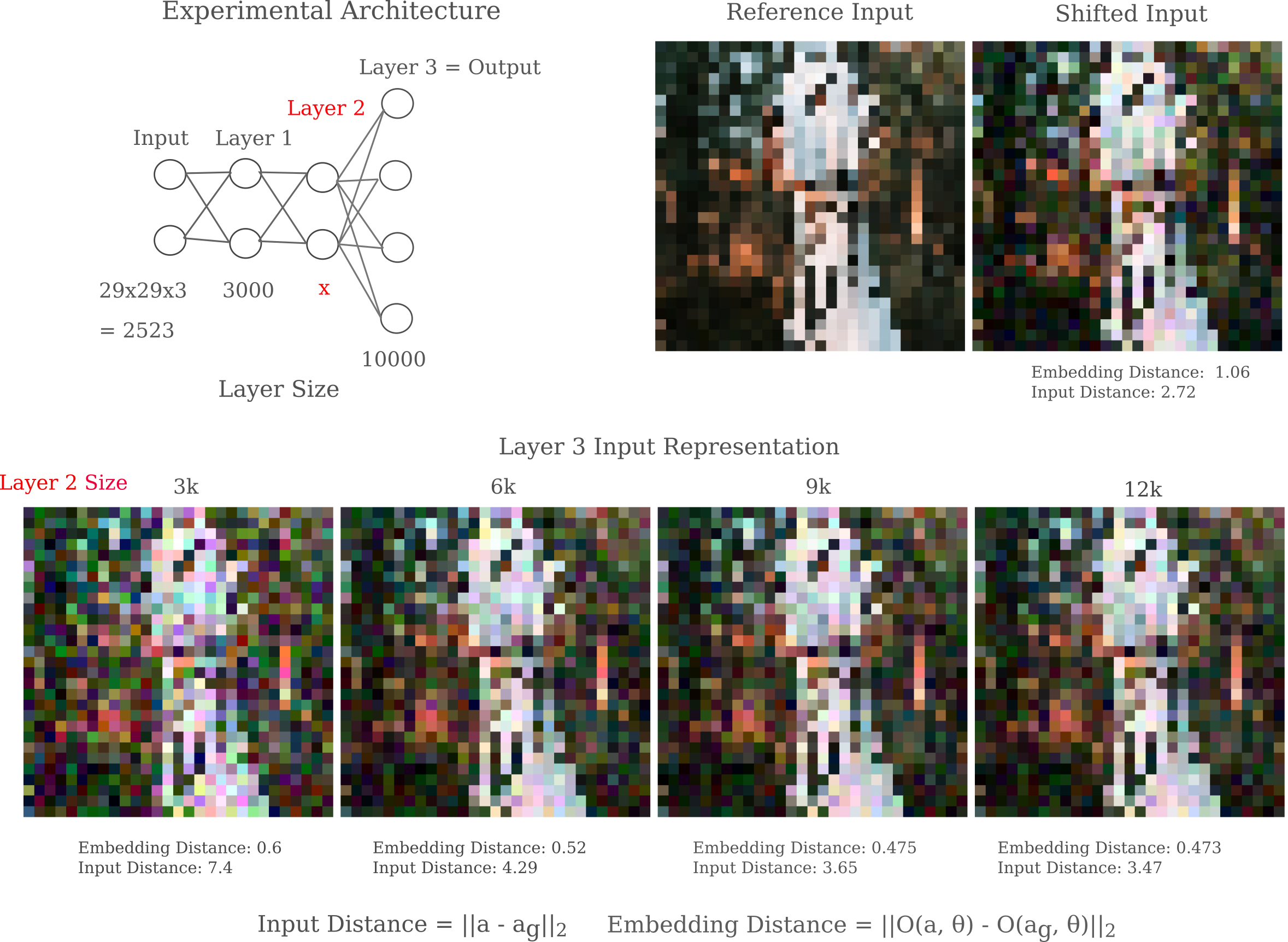
\[y = ABCDx \\\]

This theory is borne out in experimentation, where it appears impossible to make a unique trivial representation of an input of size $a$ with a layer of size $b < a$. In the following figures, the representation visualization method has been modified to have a minimum learning rate of 0.0001 and Gaussian normalization has been removed. Inputs have been down-scaled to 29x29 for fully connected model feasibility.

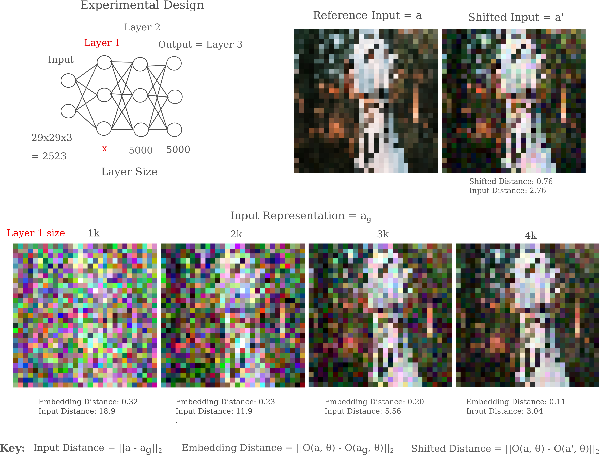
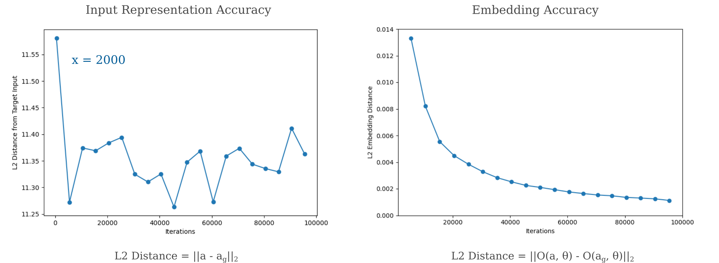
From the above figure, it may be argued that perhaps the representation generation algorithm is simply not strong enough to capture an accurate representation of the input for smaller layers. This can be shown to be not the case: plotting the representation accuracies achieved using various iterations of our representation generator, we find that only models with a minimum layer size greater than the input dimension are capable of making arbitrarily accurate representtions. For the below figure, note that if we continue to trade the 3000-width model, an exponential decay is still observed such that very low (0.1) distance is achieved after 200,000 iterations.

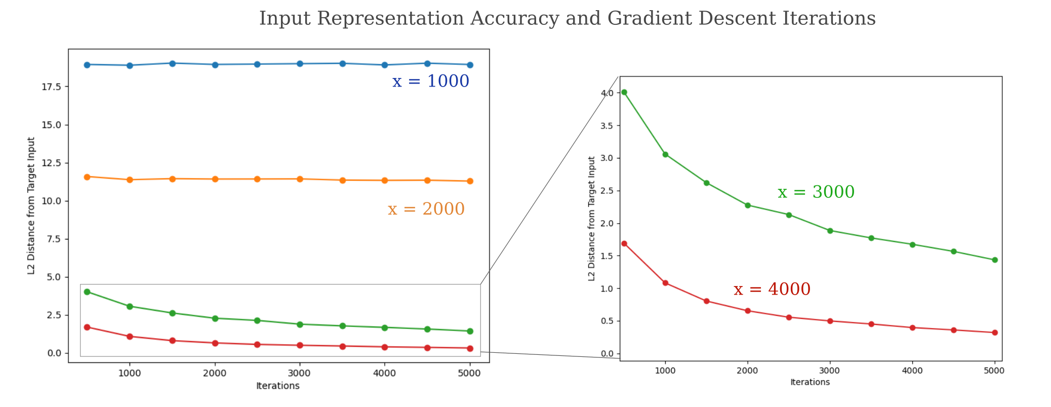
On the other hand, the 2000-width model has no decrease in distance from 1,000 to 100,000 iterations even as the embedding distance follows an exponential decay. These observations provide evidence for the idea that the input representation quality is poor for models with at least one layer with fewer nodes than input elements because of non-uniqueness rather than poor output approximation.

But something unexpected is observed for fully connected architectures in which all layers are the same size and identical (or larger than) the input: increased depth still leads to worse representational accuracy for any given number of iterations of our representation visualization method. Note that increasing the number of iterations in the representation visualization method (from 500 to 10,000 in this case) is capable of compensating for increased depth.

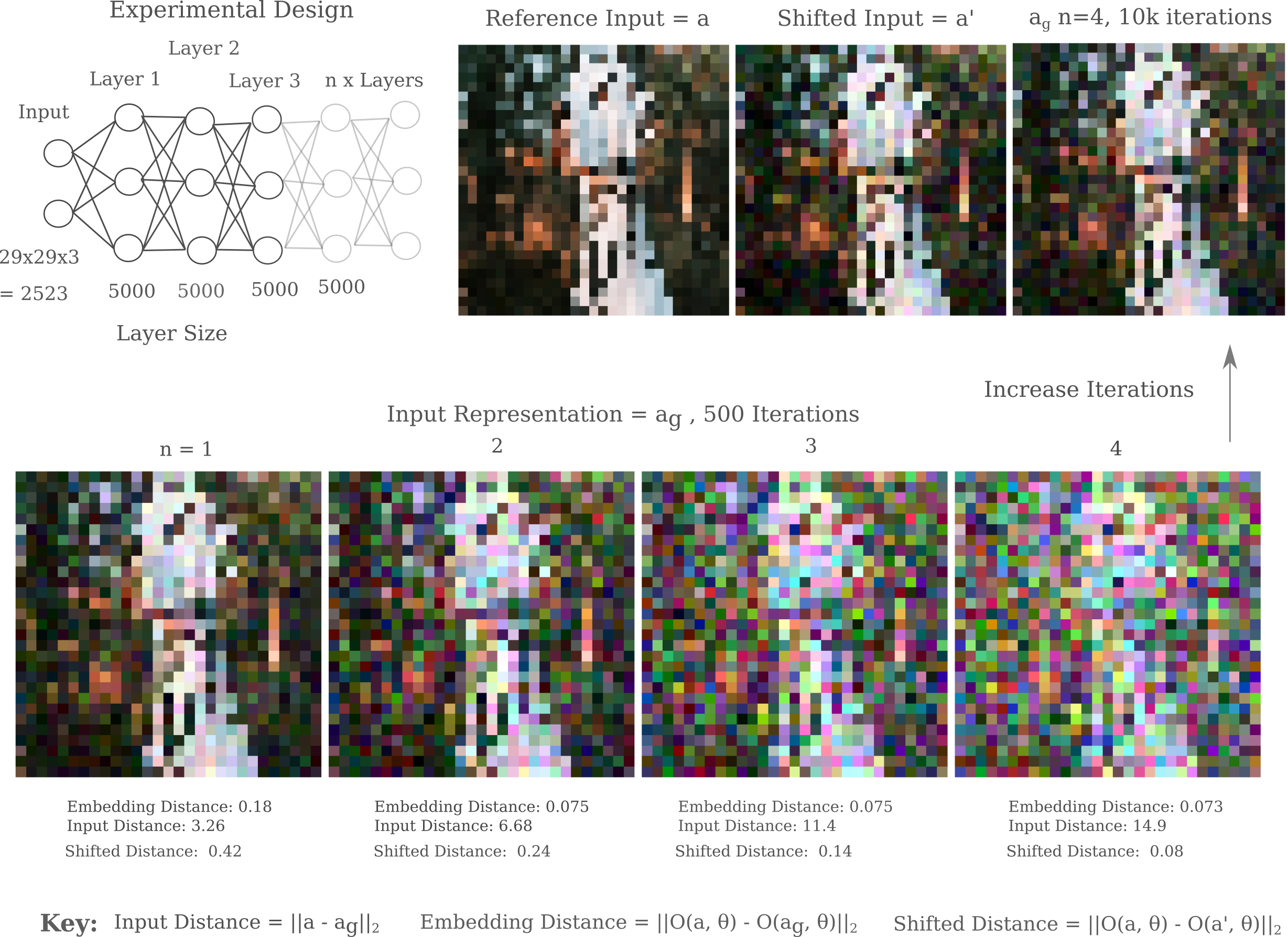
How could this be? Each layer is uniquely defined by the last, so non-uniqueness is no longer an issue. And indeed, if we increase the number of iterations of our gradient descent method for visualization the representation does indeed appear to approximate an input to an arbitrary degree. To be precise, therefore, it is observed for deep models that there are two seemingly contradictory observations:

\[m_g = ||O(a, \theta) - O(a_g, \theta)||_2 \\ m_{a'} = ||O(a, \theta) - O(a', \theta)||_2\]

we can find some input $a_g$ such that

\[m_{a'} > m_g \tag{1}\]

but for this input $a_g$,

\[|| a - a' ||_2 < || a - a_g ||_2 \tag{2}\]

which is an exact way of saying that the representation is worse even though it makes as good an approximation of $O(a, \theta)$ as $a’$.

Ignoring biases for now, fully connected linear layers are equivalent to matrix multiplication operations. If the properties of composed matrix multiplication are considered, we find that there is indeed a sufficient theory as to how this could occur. Consider first that a composition of matrix multiplications is itself equal to another matrix multiplication,

\[ABCDx = Ex\]

Now consider how this multiplication transforms space in $x$ dimensions. Some basis vectors end up becoming much more compressed or expanded than others upon composition. Consider the case for two dimensions such that the transformation $Ex$ shrinks $x_1$ by a factor of 1000 but leaves $x_2$ unchanged. Now consider what happens when we add a vector of some small amount $\epsilon$ to $x$ and find

\[|| E(\epsilon) ||\]

the difference of between transformed points $x$ and $x + \epsilon$. We would end up with a value very near $\epsilon_2$. For example, we could have

\[\epsilon = \begin{bmatrix} 1 \\ 1 \\ \end{bmatrix}\]

But now consider all the possible inputs $a$ that could make

\[|| E(a) || \approx || E(\epsilon) ||\]

If we have the vector

\[a = \begin{bmatrix} 1000 \\ 0 \\ \end{bmatrix}\]

For the choice of an $L^1$ metric, clearly

\[||E(x - a)|| = 1 < ||E(x - \epsilon)|| = 1.001\]

even though

\[||x - a|| = 1000 > 2 = ||x - \epsilon||\]

This example is instructive because it shows us how equations (1) and (2) may be simultanously fulfilled: all we need is a transformation that is contractive much more in some dimensions rather than others. Most deep learning initializations lead to this phenomenon, meaning that the composition of linear layers gives a transformation that when applied to an n-dimensional ball as an input gives a spiky ball, where the spikes correspond to dimensions that are contracted much more than others.

For an illustration of how this can occur in four dimensions, take an instance where two dimensions denoted in blue that exist on the plane of the page and two more are denoted in red, one of which experiences much more contraction than the other three. The points that will end up within a certain $L^2$ distance from the target $E(x)$ are denoted for in different dimensions by color. Two more points are chosen, one in which a small amount $\epsilon$ is added to $a$ and another which could be generated by gradient descent, $a_g$. Observe how the mapping leads to an inversion with respect to the distance between these points and $a$

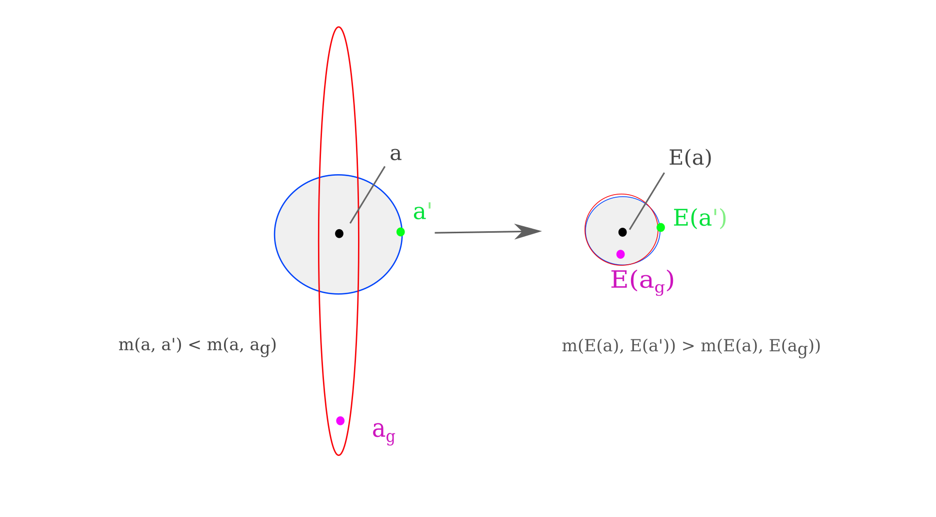
Why would a representation visualization method using gradient descent tend to find a point like $a_g$ that exists farther from $a$ than $a’$? We can think of the gradient descent procedure as finding an point $E(a_g)$ as close to $a$ as possible under certain constraints. The larger the difference in basis vector contraction that exists in $E$, the more likely that the point found $E^{-1}(a_g) = a_g$ will be far from $a$.

As the transformation $E$ is composed of more and more layers, the contraction or expansion difference (sometimes called the condition number) between different basis vectors is expected to become larger for most deep learning initialization schemes. As input representation method is very similar to the gradient descent procedure of training model parameters, poor conditioning leading to a poor input representation then it likely also leads to poor parameter updates for the early layers as well. Conditioning can be understood as signifying approximate invertibility: the poorer the conditioning of a transformation, the more difficult it is to invert accurately.

In some respects, $a’$ provides a kind of lower bound to how accurate a point at distance $E(a’) - E(a)$ could be. Observe in the figure above how small a subset of the space around $E(a)$ that $E(a’)$ exists inside. Therefore if one were to choose a point at random in the neighborhood of $E(x)$, a point like $E(a’)$ satisfying the specific conditions that it does is highly unlikely to be chosen.

This an be investigated experimentally. Ceasing to ignore biases, we can design a model such that each layer is invertible by making the number of neurons per layer equal to the number of elements in the input. We design a four-layer network of linear layers only, without any nonlinearities for simplicity. For each layer, any output $o$ will have a unique corresponding input $x$ that may be calculated by multiplying the output minus the bias vector by the inverse of the weight matrix.

\[o = Wx + b \implies \\ x = W^{-1}(o-b)\]

Inverting large matricies requires a number of operations, and it appears that the 32-bit torch.float type is insufficient for accurate inversion for the matricies used above. Instead it is necessary to use torch.double type elements, which are 64-bit floating point numbers. Once this is done, it can be easily checked that the inverse of $O(a, \theta)$ can be found.

With this ability in hand, we can investigate how likely one is to find a point within a certain distance from a target $O(a, \theta)$, denoted $O(a’’, \theta)$ such that the input is within some distance of $a$. We can do this by finding random points near $O(a, \theta)$ by

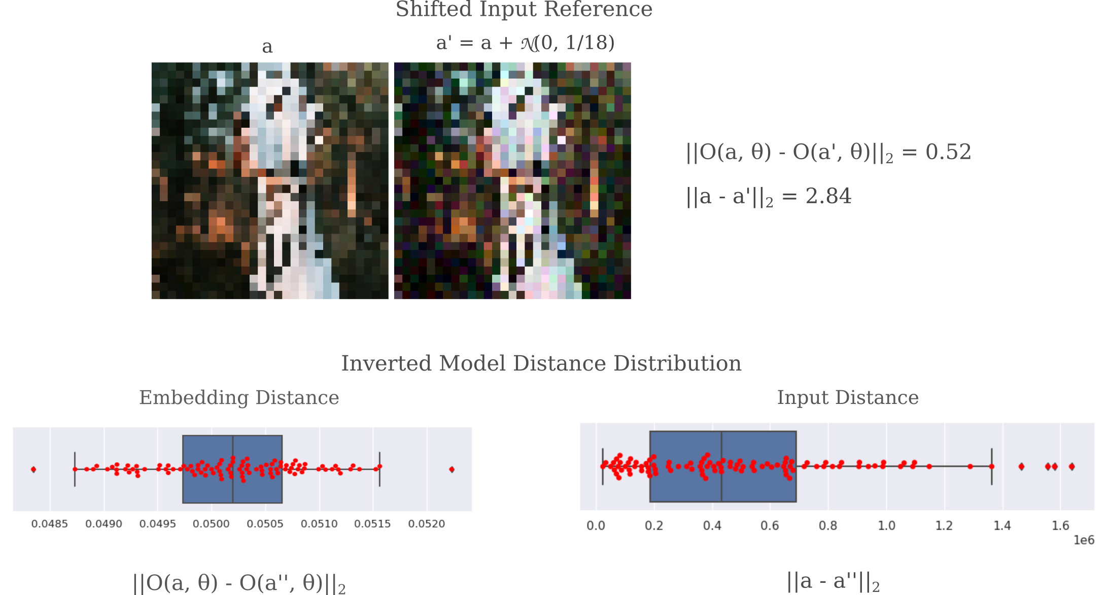
\[O(a'', \theta) = O(a, \theta) + \mathcal{N}(0, 1/1000)\]

and we can compare the distances between $a’’$ and $a$ to the distance between $a’$ and $a$. The latter is denoted in the upper portion of the following figure, and the distribution of the former in the lower portion. Observe how nearly all points $a’’$ are much farther from $a$ (note the scale: the median distance if more than 40,000) than $a’$ (which is under 3). This suggests that indeed $a’$ is unusually good at approximating $a$ for points in the neighborhood of $O(a, \theta)$, which is not particularly surprising given that $a’$ was chosen to be a small distance from $a$.

What is more surprising is that we also find that the gradient descent method for visualizing the representation of the output is also far more accurate to the orginal input $a$ than almost all other points in the neighborhood. In the below example, a short (220 iterations) run of the gradient descent method yields an input $a_g$ such that $m(a, a_g)=2.84$ for an $L^2$ metric but $m(O(a, \theta), O(a_g, \theta)) = 0.52$ with the same metric, which is far larger in output space than the neighborhood explored above but far smaller in input space.

It is worth exploring why gradient descent would yield an input $a_g$ that is much closer to $a$ than nearly all other input ${ a’’ }$ within a certain radius. Upon some close inspection, there is a clear explanation for this phenomenon: nearly all elements of ${ a’’ }$ contian pixels that are very far from the desired range $[0, 1]$ and therefore cannot be accurate input representations. Note that our gradient descent procedure was initialized with all pixels $a_0 \in \mathcal(0.7, 1/20)$ which is near the center of $[0, 1]$. Therefore it is no surprise that gradient descent starting with $a_0$ leads to an input representation $a_g$ that is much closer to the target input $a$, given that each element of the target input $a_{nm}$ also exhibits $a_{nm} \in [0, 1]$.

Theoretical lower bounds for perfect input representation

How many neurons per layer are required for perfect representation of the input? Most classification models make use of Rectified Linear Units (ReLU), defined as

\[y = f(x) = \begin{cases} 0, & \text{if $x$ $\leq$ 0} \\ x, & \text{if $x$ > 0} \end{cases}\]

In this case, the number of neurons per layer required for non-uniqueness is usually much greater than the number of input elements, usually by a factor of around 2. The exact amount depends on the number of neurons that fulfill the first if condition in the equation above, and if we make the reasonable assumption that $1/2$ of all neurons in a layer do get zeroed out then we would need twice the number of total neurons in that layer compared to input features in order to make an arbitrarily accurate representation.

This increase in the number of neurons per layer is true not just for the first but also for all subsequent layers if ReLU activation is used. This is because inverting any given layer requires at least as many unique inputs as there are previous neurons. For a probability $p$ that some chosen neuron will satisfy $y > 0$, assuming that this probability is constant for all layers we have:

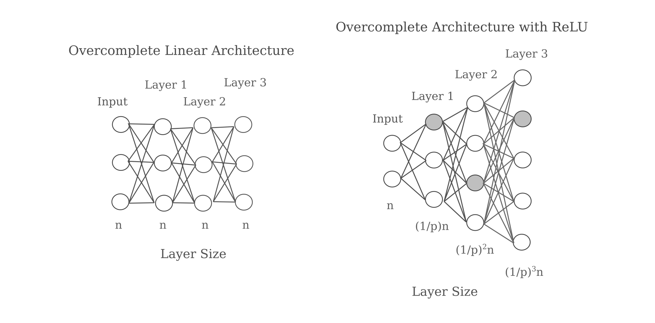
It should be noted that this phenomenon is extremely general: it applies to convolutional layers as well, and also approximately to other nonlinear activations such as tanh or sigmoid neurons. That said, however, it is by no means a given that a model will not learn to adopt some special configuration, perhaps $p=0$ such that there are no zero-valued activations per layer.

Input representations require a substantial amount of information from the gradient of the representation with respect to the input in order to make an accurate representation visualization. This means that one would ideally want to observe $a_g$ after a huge number of gradient descent steps, but for practicality iterations are usually limited to somewhere in the hundreds.

But curiously enough there is a way to reduce the number of steps necessary: add neurons to the later layers. Experimentally, increasing the number of neurons in these layers leads to a more accurate representation. As this cannot result from an increase in information during the forward pass, it instead results from a more accurate gradient passed to the input during backpropegation.

It is interesting that increasing the number of deep layer neurons is capable of leading to a better input representation for a deep layer even for overcomplete architectures with more layer neurons than input elements. It is probable that increased deep layer neurons prevent scaling problems of gradients within each layer.

In conclusion, poor representation of an input may be due to non-uniqueness caused by non-invertible functions commonly used in models in addition to poor conditioning (which can be thought of as approximate non-invertibility) resulting in difficulties of sufficiently approximating $O(a, \theta)$. For ResNet, it appears that the non-uniqueness phenomenon is the root of most of the inaccuracy in deep layers’ representations due to the observation that input distance tends to increase while embedding distance decreases upon better and better embedding approximation.

There one final piece of evidence for non-uniqueness being the primary cause of poor representation. Observe that the representation for ResNet50 layer Conv1 before batchnorm and max pooling (trained or untrained) is near-perfect, whereas the representation after applying batchnorm and more importantly pooling is not (especially for the untrained model). This is precisely what is predicted by the non-uniqueness theory, as the first convolutional layer input contains $299x299x3 = 268,203$ elements and the output has over one million and thus is invertible, but the addition of max pooling leads to non-invertibility.

The effect of training on layer approximation accuracy

What happens to the poor representations in deeper layers upon model training? We have already seen that training leads to the formation of what was termed a non-trivial representation, ie something that is not simply an approximate copy of the input. The human eye can distinguish recognizable features of this representation if Gaussian blurring is used during gradient descent. It may be illuminating to investigate how training changes or does not change the ability of a deep layer to represent an input.

As it is extremly unlikely that training would lead to the transformation of $O(a, \theta)$ from the spiky ball geometry to a non-spiky ball (ie lower the condition number ro near unity), and it is not possible for training to remove the non-uniqueness of a representation for any given output, one would expect for the same disconnect between embedding and input distances upon increased iterations of gradient descent. Indeed this is observed, as for example for layer Conv5 of a trained ResNet50 exhibits the same inverse correlation between input and embedding distances as the untrained ResNet50 model does.

Therefore training does not change the underyling inability in forming an accurate representation of an input for deeper layers. But it may change the ease of approximating those representations. Successful training leads to a decrease in some objective function $J(O(a, \theta))$ such that some desired metric on the output is decreased. It may be hypothesized that training also leads to a decrease in the distance between the representation of the generated input $a_g$ and the representation of the actual input $a$ for some fixed number of iterations of our representation method. For representations without Gaussian convolutions applied at each step, this does appear to be the case.

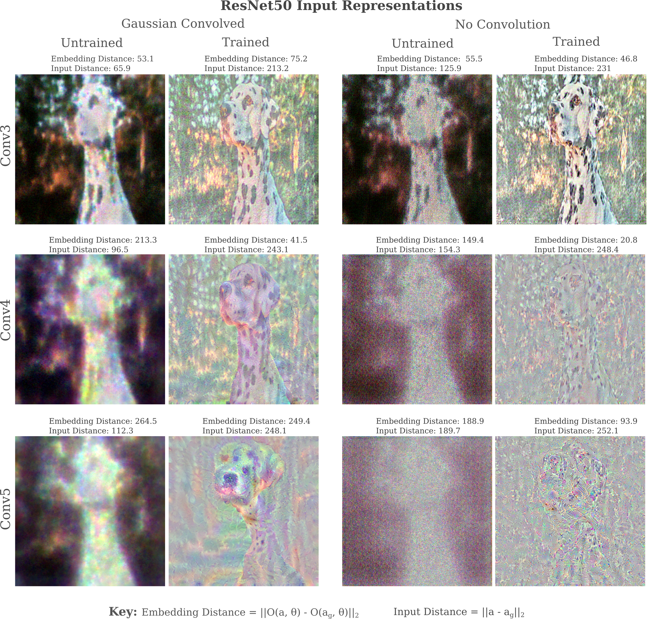
Upon close examination of the trained versus untrained early and middle layers of ResNet50, however, training leads to a representation of the input that is noticeably sharper than for the untrained case. It may be wondered if representations of images that would not be recognized by a model trained on Imagenet would also be sharpened or not. This may be explored by observing the clarity of representations $a_g$ for an image of a Tesla Coil at different layers. We find that indeed input representations early and middle layers of ResNet50 are sharpened upon training.

This observation gives a hypothesis as to why the feature maps for early layers are repeating pattern, as observed here. The parameters of these layers are capable of learning to restrict the possible representations of the input to be sharp images that retain most of the detail in the input.

It has ben observed that kernals of convolutional models applied to a wide range of image-recognition tasks tend to form Gabor filters. These filters are the product of sinusoidal functions with Gaussians and are used for (among other purposes) edge detection. It has been suggested that these filters allow early convolutional layers to perform selection for simple features such as edges, which is followed by selection for objects of greater abstractions in later layers.

This perspective undoubtedly has merit, but we can provide a different one: early layers learn convolutional weights that serve to restrict the possible inputs that could yield a similar representation in that layer, which leads to the visualization of that representation becoming visually sharpened and more clear in certain areas of the input. What is sharpened and what is not can be gradually selected for in each layer such that the model only allows information to pass to the output if it is important for classification.

In conclusion, the generated input representation $a_g$ does indeed change noticeably during training, but that this change does not affect the tendancy for deep layers to lack uniqueness in their representations. Indeed this is clear from the theory expoused in the last section, as the convolutional operation remains non-invertible after training and the spiky ball geometry would not necessarily be expected to disappear as well.

Instead, it appears that during training the possible inputs that make some representation close to the target tensor are re-arranged such that the important pieces of information (in the above case the snout and nose of a dog) are found in the representation, even as non-uniqueness remains. And indeed this would be expected to be helpful for the task of input classification, as if the classification output for some hidden layer’s activation vector $h = O(a, \theta)$ is correct then all inputs that map to this value $h$ would also be correct.

Late layer representations are mostly inference

In various cases it is clear that early convolutional layers learn to more precisely represent the input, whereas later layers introduce new information as to what the input should be (rather than is). This is apparent for the image of the Dalmatian in which the spot pattern changes noticeably in middle layers and in later layers that exaggerate the snout.

This question may be addressed by training ResNet50 to recognize images of random noise. In this experiment, 10,000 images of random scaled Gaussian noise $\mathcal{N}(1/2, 1/4)$, each sample labelled as one of 100 categories. As seen in other work, deep learning vision models are somewhat surprisingly capable of accurately classifying these images of noise. An example input is as follows:

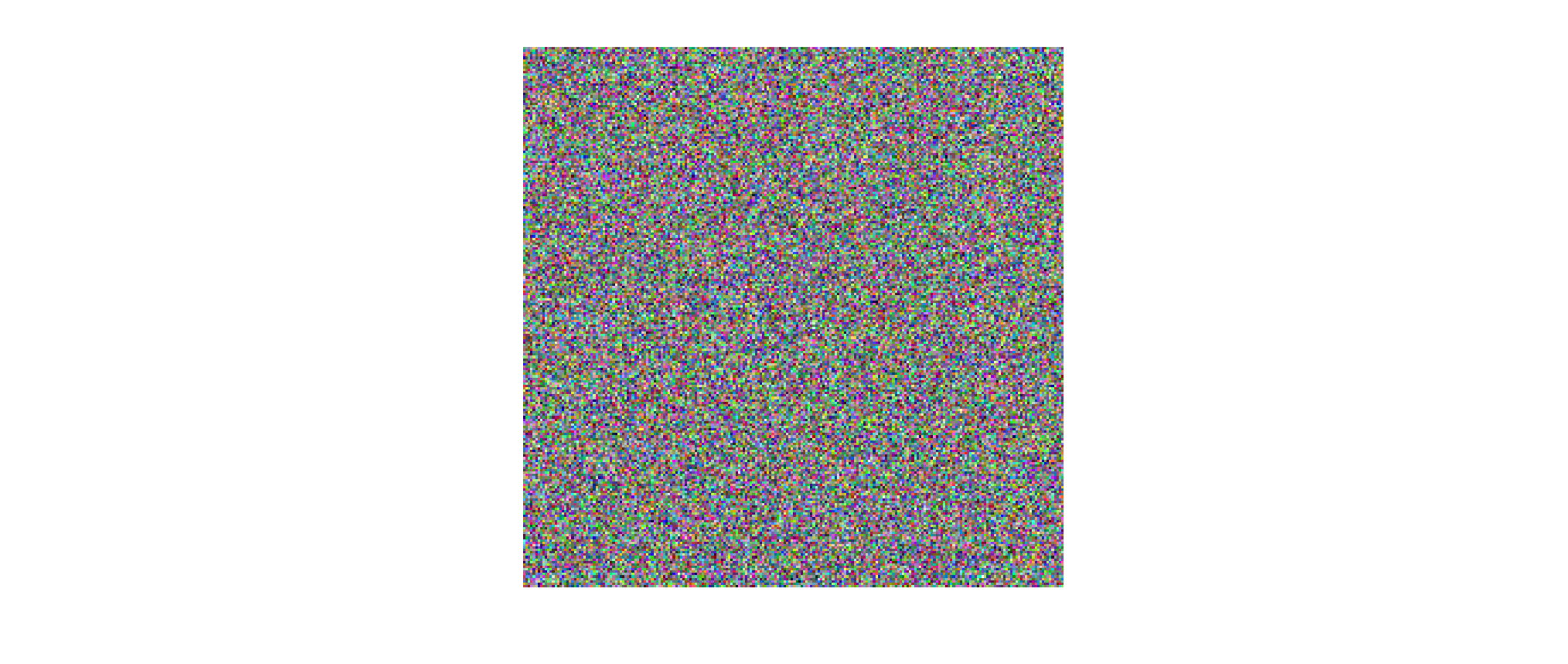
It is clear that attempting to classify thousands of such images requires memorizing each one, which is extremely difficult to do for the human visual system, although it is abundantly easy for deep learning vision models such as ResNet. This suggests that the process of image recognition is fundamentally different for natural images compared to random ones, and we might expect that difference to manifest itself in the representations that a random-trained model forms of a natural image.

Applying gradient descent to form input representations of the embeddings at various layers for a random-trained ResNet50, we see that indeed the information is much different than for ResNet50 trained on ImageNet. The process of generating an input is noticably changed: applying a Gaussian convolution to smooth the representation results in inputs $a_g$ that do not approximate the input’s embedding as well as $O(a’, \theta)$. To be specific,

\[||O(a, \theta) - O(a_g, \theta)|| > ||O(a, \theta) - O(a', \theta)||\]

for $\theta$ trained on noise and $a_g$ generated using Gaussian convolutions at each gradient update step, with $a’$ being the shifted version of $a$ noted in previous sections.

This contrasts with input representations for ResNet50 trained on ImageNet in which it is straightforward to find an $a_g$ such that

\[||O(a, \theta) - O(a_g, \theta)|| < ||O(a, \theta) - O(a', \theta)||\]

even for a limited number of gradient descent steps. But when one considers the dataset that $\theta$ was trained on, this finding is not surprising: the training input are not smooth and unlike natural images would be poorly approximated by Gaussian-convolved versions.

Commensurately, if apply the gradient descent procedure without Gaussian convolution we find that obtaining a $a_g$ that yields an output that approximates $O(a, \theta)$ better than $O(a’, \theta)$ is not difficult. But the results look nothing like the case for models trained on imagenet: layers Conv3 through Conv5 contain almost no information on the input but rather infer that it must resemble the random training data seen by this model.

It can also be appreciated that the early layer representations are not noticeably clearer after training on random inputs compared to the untrained model. In the following figure Gaussian convolution was performed at each gradient descent step for consistency.

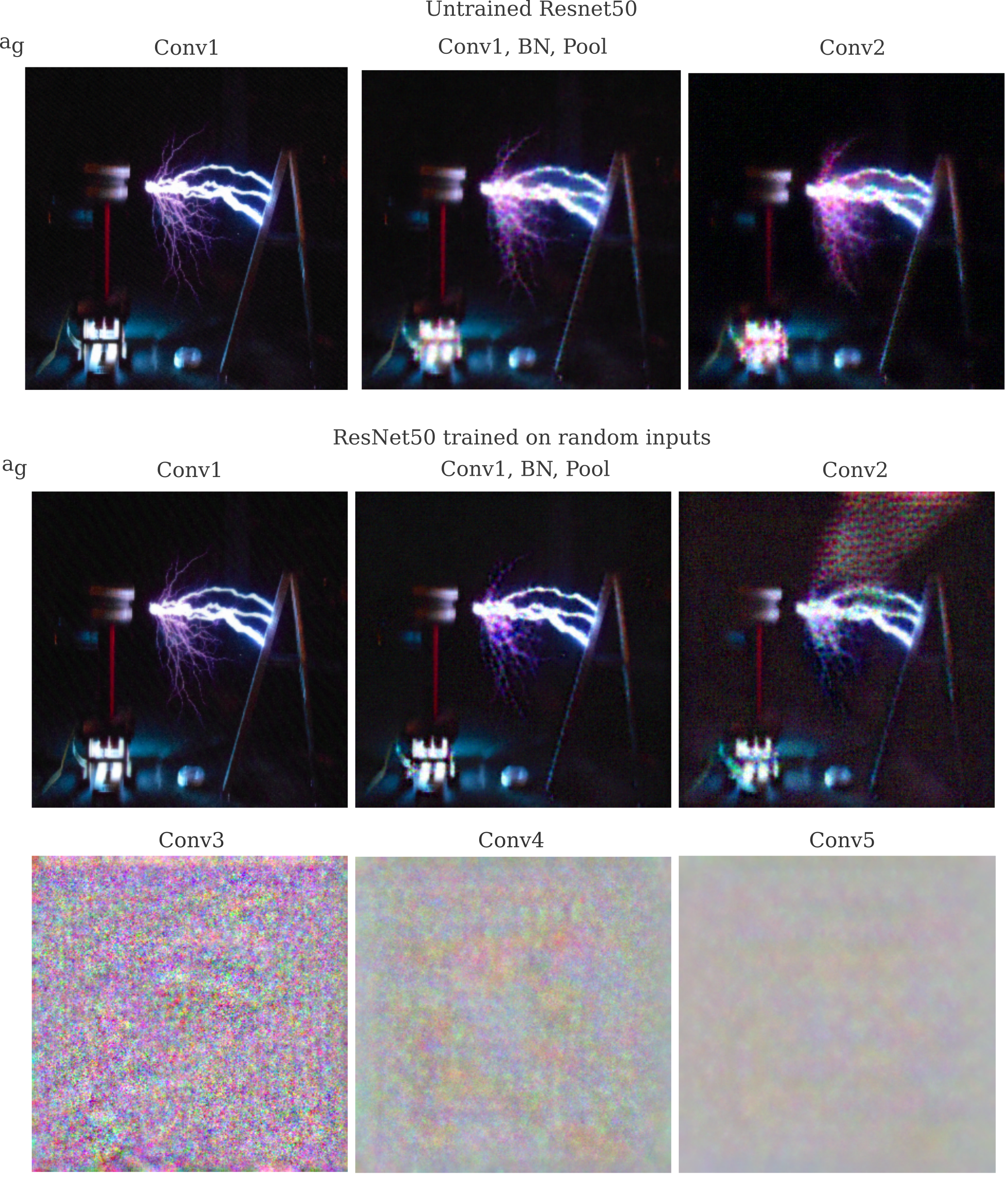
From these observations can be drawn two conclusions: first that representations in later layers reflect the training dataset’s content far more than the input itself, and second that the tendancy of early layer representations to become visually sharpened (via restriction of possible feasible inputs) is specific to tasks using natural images rather than existing in every trained model regardless of training dataset.

Implications of imperfect input representation

For models applied to the task of classification, particularly where there are fewer classification categories than input elements, then necessarily all the information from the input does not reach the output such that backpropegation cannot instruct the network to exactly copy an input (in the general case, barring certain weight and bias configurations). But for hidden state models or for classification in which there are many more output elements than inputs, exact representation becomes important.

The theory developed on this page also gives an explanation for the common architecture for autoencoders. Typically these seek to avoid copying the input to the output and thus have fewer elements in the latent space than inputs. On the other hand, they also typically do not want to lose information between the latent space and output, which may be why an increasing-size architecture has been found to be so successful.

The theory of representation accuracy goes some way towards explaining the types of architectures that have been found to be successful in a variety of tasks in recent times as well. Transformers use stacks of self-attention and feed-forward fully connected units to create representations of inputs, both of which are typically non-invertible (for example see that a single self-attention output vector value can be any linear combination of softmax outputs of $q*k$ values at each input). Alternatives to transformers that have also proven effective in recent years combine fully connected subcomponents in non-invertible methods (for example the mlp-mixer architecture’s output can be a linear combination of any given weight vector). It remains to be seen, however, whether or not vision transformers and MLP-mixers (and in general any patch-based method) tend to learn to sharpen the input before mapping it to a manifold as occurs for convolutional models.