Input Generation III: Model Similarity and Autoencoding Representations

Model Similarity Vector Space

In part I, it was observed that different models generate slightly different representations of each ImageNet input class. It may be wondered whether or not we can use the gradients of two models to make an input, perhaps by combining the gradients of a model with parameters $\theta_1$ and another with parameters $\theta_2$ to make a gradient $g’$

\[g' = \nabla_a \left( d(C - O_i(a, \theta_1)) + e(C - O_i(a, \theta_2)) \right)\]

where $d, e$ are constants used to scale the gradients of models $\theta_1, \theta_2$ appropriately. For GoogleNet and Resnet, we approximate $d = 2, e = 1$ by applying the constant only to $C$ as follows (note that there is little difference in applying the constant to the gradient or the constant alone)

def layer_gradient(model, input_tensor, desired_output):
    ...
    loss = 0.5*((200 - output[0][int(desired_output)]) + (400 - output2[0][int(desired_output)]))
    ...

where output is the (logit) output of ResNet and output2 is the output from GoogleNet.

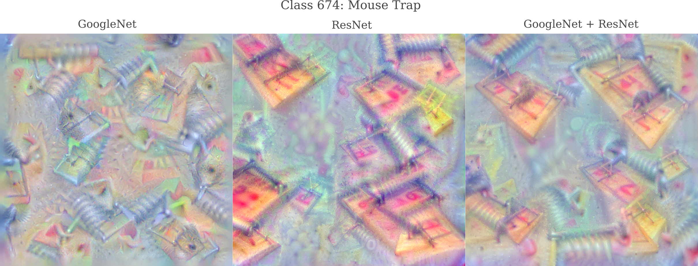
Images of all 1000 ImageNet classes generated using the combined gradient of GoogleNet and ResNet are available here. From these images it is clear that the combined gradient is as good as or superior to the gradients from only ResNet or GoogleNet with respect to producing a coherent input image, which suggests that the gradients from these models are not substantially dissimilar.

The above observation motivates the following question: can we attempt to understand the differences between models by generating an image representing the difference between the output activations for any image $a$? We can construct a gradient similar to what was employed above,

\[g'' = \nabla_a \left( d(C - O_i(a, \theta_1)) - e(C - O_i(a, \theta_2)) \right)\]

again with output and output2 signifying the logit output from ResNet and GoogleNet, respectively.

def layer_gradient(model, input_tensor, desired_output):
    ...
    loss = 2*((200 - output[0][int(desired_output)]) - (400 - output2[0][int(desired_output)]))
    ...

Which yields

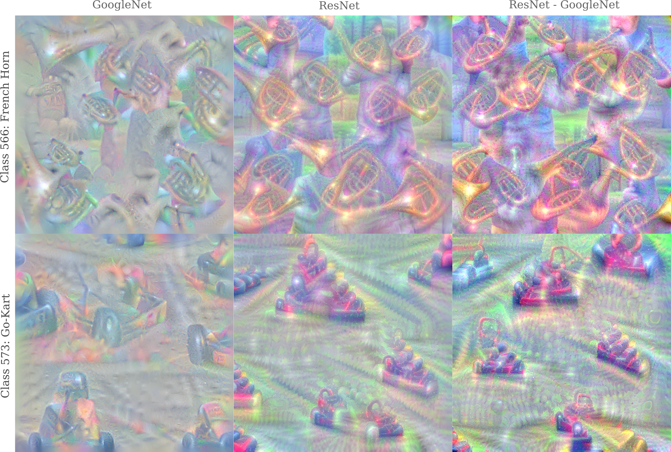
Note that the roll-over bars present in the depiction of go-karts by ResNet50 are absent for GoogleNet’s representation of the same class, and that consequently the representation using $g’’$ exaggerates this feature. The same exaggeration of features not found in GoogleNet’s but that are found in ResNet’s representation of a french horn (mostly the figures playing the instruments) is also observed.

For other ImageNet classes, however, there does not tend to be a substantial difference between inputs generated for each class via applying the gradient $g$ of ResNet50 compared to $g’’$. It is likely that this is because minimizing the activation for some particular class does not yield enough information to generate an input in certain cases. For an in-depth investigation into generating the inputs corresponding to the subtracted term of $g’’$, see this page.

It is also apparent that the similarities and differences in model output may be compared by viewing the output as a vector space. Say two models were to give very similar outputs for a representation of one ImageNet class but different outputs for another class. The identities of the classes may help inform an understanding of the the difference between models.

Model Merging

In the last section it was observed that we can understand some of the similarities and differences between models by viewing the output as a vector space, with each model’s output on each ImageNet representation being a point in this space.

What if we want one model to generate a representation of an ImageNet class that is similar to another model’s representation? We have already seen that some models (GoogleNet and Resnet) generally yield recognizable input representations whereas others (InceptionV3) yield somewhat less-recognizable inputs. But if we were stuck with only using InceptionV3 as our image-generation source, can we try to use some information present from the other models in order to generate a more-recognizalbe image?

One may hypothesize that it could be possible to train one model to become ‘more like’ another model using the output of the second as the target for the output of the first. Consider one standard method of training using maximum likelihood estimation via minimization of cross-entropy betwen the true output $Q$ and the model output $Q$ given input $x$,

\[J(O(a, \theta), \widehat y) = H(P, Q) = -\Bbb E_{x \sim P} \log Q(x)\]

The true output $Q$ is usually denoted as a one-hot vector, ie for an image that belongs to the first ImageNet category we have $[1, 0, 0, 0…]$. A cross-entropy loss function measures the similarity between the output distribution model output $Q$ and this one-hot tensor $Q$.

But there are indications that this is not an optimal training loss. Earlier on this page we have seen that for trained models, some ImageNet categories are more similar with respect to the output activations $O(a, \theta)$ to some other ImageNet categories, and different from others. These similarities moreover are by a nearest neighbors graphical representation intuitive for a human observer, meaning that it is indeed likely that some inputs are more similar than others.

Training requires the separation of the distributions $P_1, P_2, … P_n$ for each imagenet category $n$ in order to make accurate predictions. But if we have a trained model that has achieved sufficient separation, the information that the model has difficulty separating certain images from others (meaning that these are more similar ImageNet categories by our output metric) is likely to be useful information in training a model. This information is not likely to be found prior to training, and thus is useful for transfer learning.

These observations motivate the hypothesis that we may be able to use the information present in the output of one model $\theta_1$ to train another model $\theta_2$ to be able to represent an input in a similar way to $\theta_1$. More precisely, one can use gradient descent on the parameters of model 1, $\theta_1$ to make some metric between the outputs $m(O(a, \theta_1), O(a, \theta_2))$ as small as possible. In the following example, we seek to minimize the sum-of-squares residual as our metric

\[J(O(a, \theta_1) = \sum_i \left(O_i(a, \theta_1) - O_i(a, \theta_2) \right)^2\]

which can be implemented as

def train(model, input_tensor, target_output):
    ...
    output = model(input_tensor)
    loss = torch.sum(torch.abs(output - target_output)**2) # sum-of-squares loss
    optimizer.zero_grad() # prevents gradients from adding between minibatches
    loss.backward()
    optimizer.step()
    return 

Note that more commonly-used metrics like $L^1$ or $L^2$ empirically do not lead to significantly different results as our RSS metric here. Whichever objective function is chosen, it can be minimized by gradient descent on the model parameters given an input image $a$ is

\[\theta_1'= \theta_1 + \epsilon * \nabla_{\theta_1} J(O(a, \theta_1))\]

which may be implemented as

def gradient_descent():
    optimizer = torch.optim.SGD(resnet.parameters(), lr=0.00001)
    # access image generated by GoogleNet
    for i, image in enumerate(images):
        break 
    image = image[0].reshape(1, 3, 299, 299).to(device)
    target_output = googlenet(image).detach().to(device)
    target_tensor = resnet(image) - target_output
    for _ in range(1000):
        train(resnet, image, target_output)

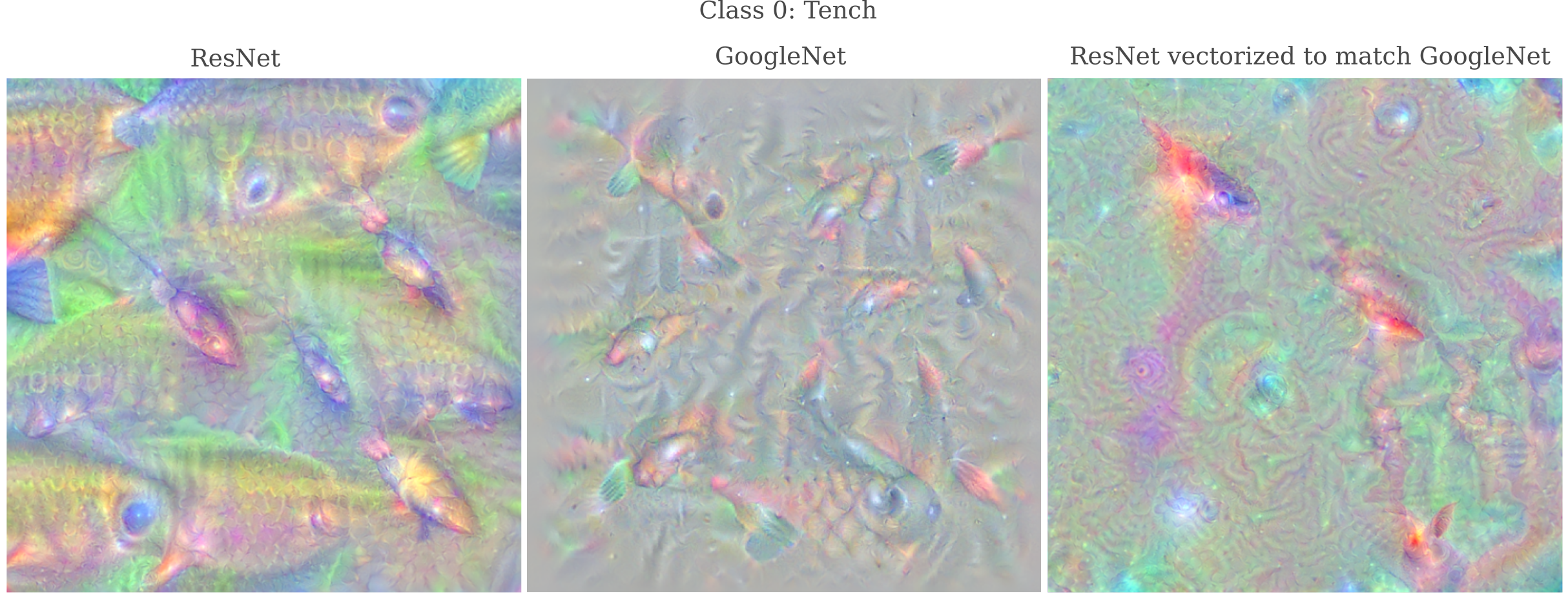
Gradient descent is fairly effective at reducing a chosen metric between ResNet $\theta_1$ and GoogleNet $\theta_2$. For example, given $a$ to be GoogleNet’s representation of Class 0 (Tench), $J(O(a, \theta_1))$ decreases by a factor of around 15. But the results are less than impressive: applying gradient descent to ResNet’s parameters as $\theta_1$ to reduce the sum-of-squares distance between this model’s output and GoogleNet’s output does not yield a model that is capable of accurately representing this class.

It may be hypothesized that this could be because although ResNet’s outputs match GoogleNet’s for this class, each class has a different ‘meaning’, ie latent space location, which would undoubtedly hinder our efforts here. But even if we repeat this procedure to train ResNet’s outputs match GoogleNet’s(for that model’s representations) for all 1000 ImageNet classes, we still do not get an accurate representation of Class 0 (or any other class of interest).

It is certainly possible that this method would be much more successful if applied to natural images rather than generated representations. But this would go somewhat against the spirit of this hypothesis because natural images would bring with them new information that may not exist in the models $\theta_1, \theta_2$ even if the images come from the ImageNet training set.

These results suggest that modifying $\theta_1$ to yield and output that matches that of $\theta_2$ is a somewhat difficult task, at least if we limit ourselves to no information that is not already present in the model. But this could simply be due to known difficulties in model training rather than an inability to explore the output latent space.

Therefore a more direct approach to making one model yield another model’s representations: rather than modifying the first model’s parameters $\theta_1$ via gradient descent, we instead find the coordinates of the second model’s representation of a given class in our output space and then use these coordinates as a target for gradient descent on an initially randomized input $a_0$.

For clarity, this procedure starts with an image representing the representation of a certain class with respect to some model $\theta_2$, denoted $a_{\theta_2}$. We want to have a different model $\theta_1$ learn how to generate an approximation of this representation with no outside information. First we find a target vector $\widehat{y} \in \Bbb R^n$, with $n$ being the number of possible outputs, defined as

\[\widehat{y} = O(a_{\theta_2}, \theta_1)\]

or in words the target vector is the output of the model of interest $\theta_1$ when the input supplied is the representation of some class for the model we want to emulate.

Now rather than performing gradient descent using a target $C \in \Bbb R^n$ being a vector with a large constant in the appropriate index for our class of interest and zeros elsewhere, we instead try to reduce the distance between $O(a_0, \theta_1)$ and the target vector $\widehat{y}$. Again this distance can be any familiar metric, perhaps $L^1$ which makes the computation as follows:

\[g = \nabla_a \sum_n \lvert \widehat{y_n} - O_n(a, \theta_1) \rvert \\\]

with the input modification being a modified version of gradient descent using smoothness (ie pixel cross-correlation) via Gaussian convolution $\mathcal{N}$ and translational invariance with Octave-based jitter, here denoted $\mathscr{J}$, were employed with the gradient for input $a_n$, denoted $g_n$. The actual update procedure is

\[a_{n+1} =\mathscr{J} \left( \mathcal{N}(a_n + \epsilon g_n) \right)\]

where the initial input $a_0$ is a scaled random normal distribution. This gradient can be implemented as follows:

def layer_gradient(model, input_tensor, desired_output):
    ...
    input_tensor.requires_grad = True
    output = resnet(input_tensor)
    loss = 0.05*torch.sum(torch.abs(target_tensor - output))
    loss.backward()
    gradient = input_tensor.grad

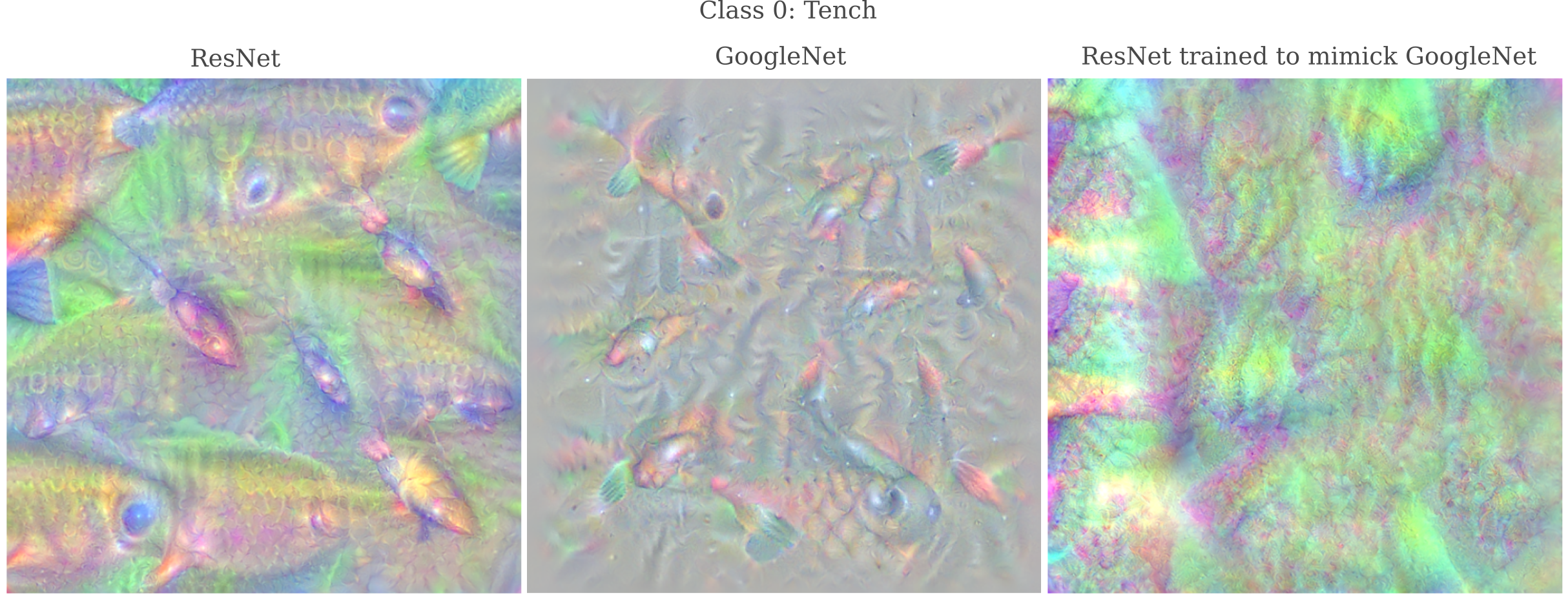
If this method is successful, it would suggest that our model of interest $\theta_1$ has the capability to portray the representation that another model $\theta_2$ has of some output class, and that this portrayal may be made merely by finding the right point in the output space. And indeed for Class 0 this is the case: observe how the output on the right mimicks GoogleNet’s representation of a Tench.

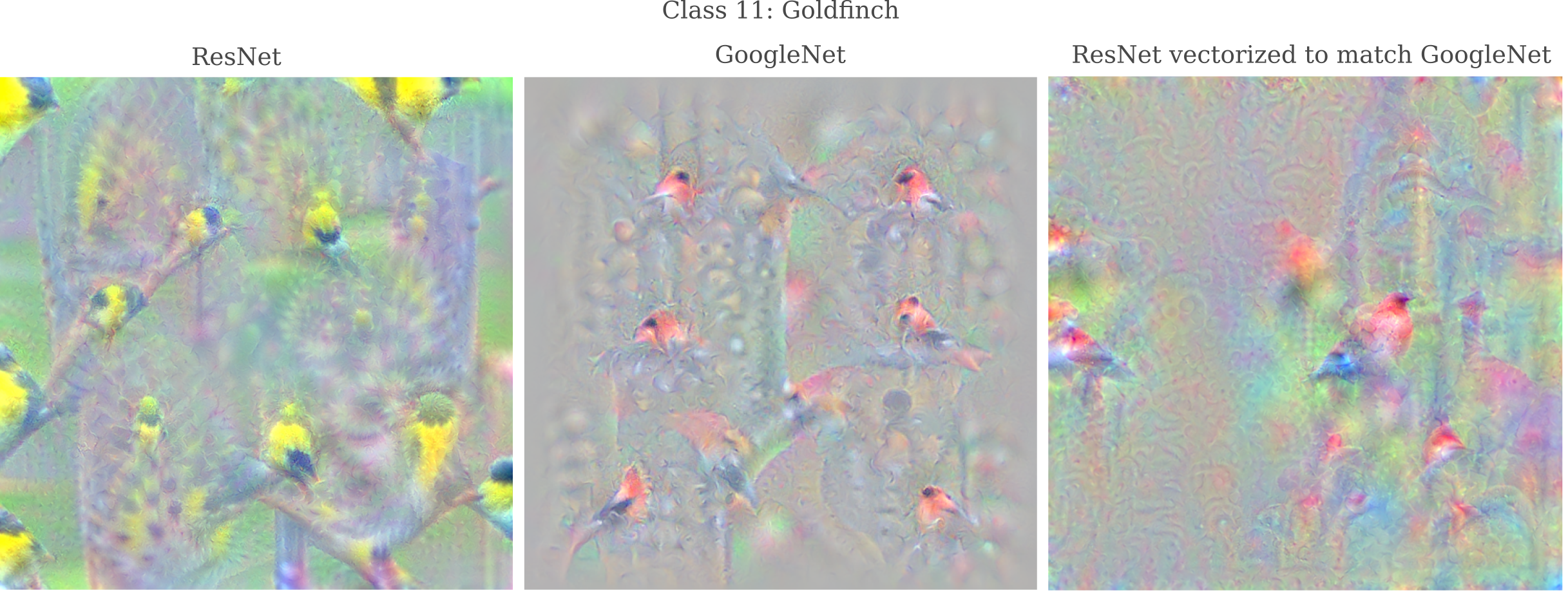
The ability of the right point in output space to mimick the representation by another model (for some given class) is even more dramatic when the model’s representations of that class are noticeably different. For example, observe the representation of ‘Class 11: Goldfinch’ by ResNet and GoogleNet in the images on the left and center below. ResNet (more accurately) portrays this class using a yellow-and-black color scheme with a dark face whereas GoogleNet’s portrayal has reddish feathers and no dark face. But if we perform the above procedure to ResNet, it too mimicks the GoogleNet output.

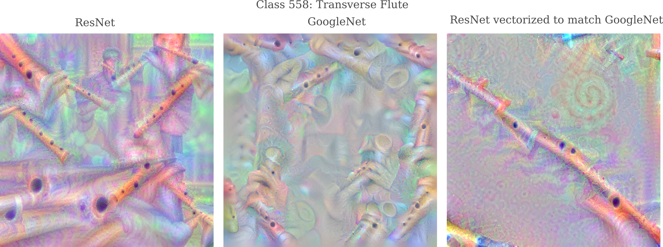
Likewise, ResNet’s depiction of a transverse flute contains flute players in addition to the instrument itself, whereas GoogleNet’s depiction does not. When we vectorize ResNet’s output to match that of GoogleNet, we see that ResNet’s depiction of a transverse flute no longer contains the players.

Natural Image Representation

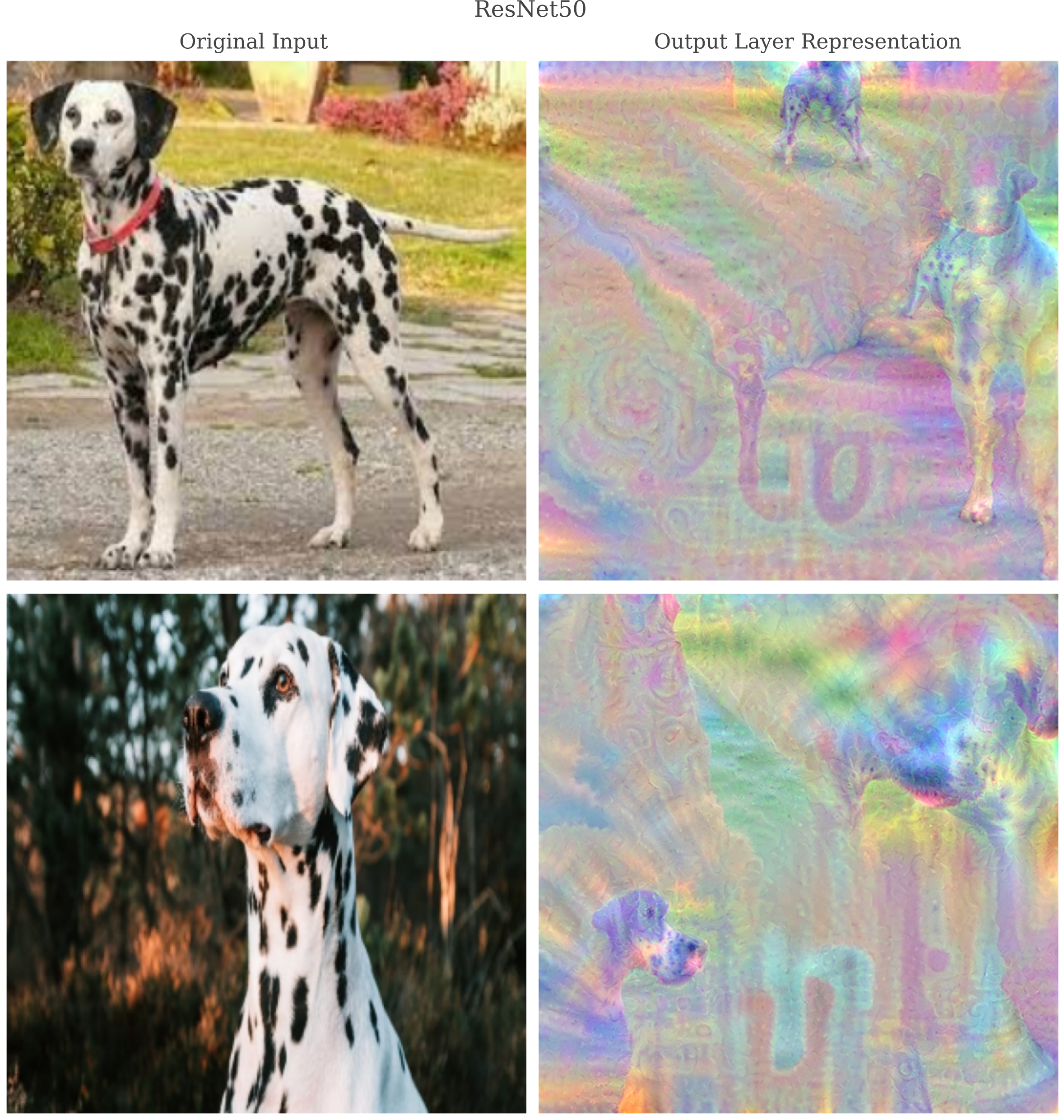
It may be wondered whether we can apply our gradient descent method to form representations of natural images, rather than generated ones representing some ImageNet category. All that is required is to change $a_{\theta_2}$ to be some given target image $a_{t}$ before performing the same octave-based gradient descent procedure.

When we choose two images of Dalmatians as our targets, we see that the representations are indeed accurate and that the features they portray are significant: observe how the top image’s representation focuses on the body and legs (which are present in the input) whereas the bottom focuses on the face (body and legs not being present in the input).