Input Generation II: Vectorization and Latent Space Exploration

This page is part II on generating inputs using deep learning models trained for image classification. For part I, follow this link. For part III, see here

Introduction with Opposites

It is remarkable that deep learning models tasked with image classification are capable of producing coherent images representing a given output class. The task of image generation is far different than classification, but nevertheless recognizable images may be generated by optimizing the output for a given class. In a previous section on this page, we also saw that images may be generated with a linear combination of two classes, which allowed us to transform a generated image of a husky into an image of a dalmatian.

These observations lead to a natural idea: perhaps we can treat the output tensor of a deep learning model as a latent space. A latent space, also known as an embedding, is informally a space that captures meaningful information about the possible objects in that space. More precisely, it is a manifold in which object similarity correlates with a distance metric on that manifold.

We will consider the final 1000-dimensional fully connected layer activation of possible ImageNet categories as the output in question. At first glance it is not clear that this could be any kind of latent space: during training, each category is denoted by a one-hot vector in this space such that all possible categories are the same distance apart from each other. This means that there is no prior information encoded in one output class versus another, which is exactly what one wants when training for classification without prior knowledge.

On the other hand, within this 1000-dimensional space we can view each class as a basis vector for this space and instead consider the possible vectors that exist in this space. A meaningful vector space of the outputs allows us to explore interesting questions by simply converting each question into a vector arithmetic operation.

On a memorable episode of the popular comedy ‘Seinfeld’, the character George decides to do the opposite of what he would normally do with appropriately comedic results. But one might wonder: what is the opposite? For a number of ideas, there seems to be a natural opposite (light and dark, open and closed) but for others ideas or objects it is more difficult to identify an opposite: for example, what is the opposite of a mountian? One might say a valley, but this is far from the only option. Likewise, objects like a tree and actions like walking do not have clear opposites.

In part I we saw that deep learning models are capable of forming an image that represents some target output $\widehat y$. This target output was usually a vector in which the entry at the index (signifying the ImageNet class) of choice was a large constant and zeros everywhere else, and the input image was modified using gradient descent in order to miminize the loss metric between the output and the target output. With certain restrictions on how the gradient can be applied (smoothness in the input, for example) coherent and recognizable images can be generated. Observation of the outputs shows that indeed the class of interest is maximized, as for example GoogleNet applied to maximize the activation of element 920 (signifying ‘stoplight’)

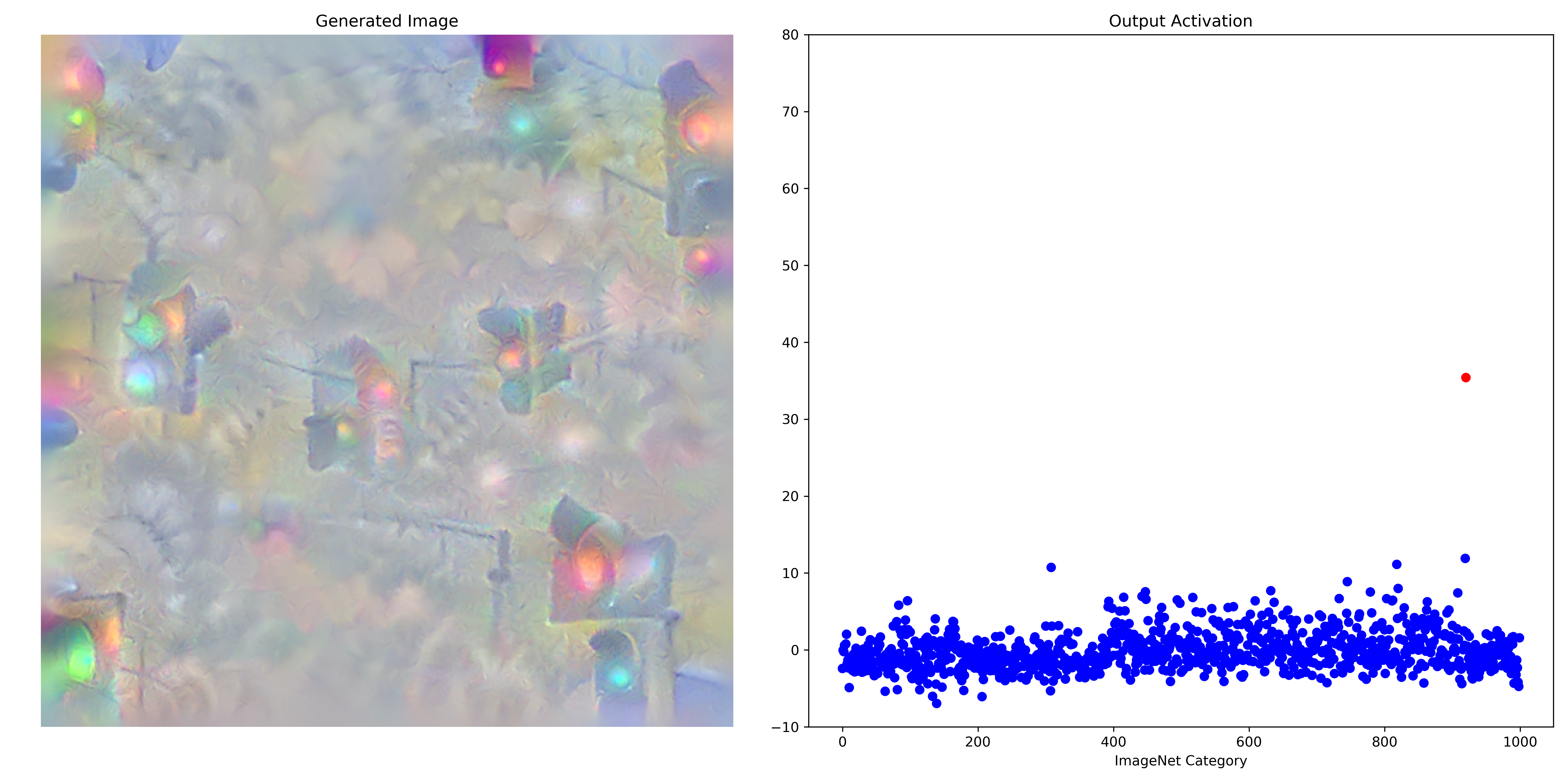
Observe that even though only index 920 was optimized, other output class activations have been affected as well. It may be hypothesized that these activations correspond to a similarity between each of the 999 other ImageNet categories and class 920, with a higher activation signifying a more similar class where ‘similar’ is a measure on the function $f$ representing the GoogleNet model. As a similarity metric this measure is actually quite effective (see the below section for more information) and it may be wondered whether the element with the smallest activation could be an accurate representation of an ‘opposite’ to the class being maximized.

More formally, we want to find the index $k$

\[k = \mathrm{arg} \; \underset{i} {\mathrm{min}} \; O_i(a; \theta)\]

where $a$ is an input generated to maximize some output class and $\theta$ denotes the configuration and parameters of the model used.

The above method does not empirically yield very interesting results: the opposites of many ImageNet categories tend to be only a few classes, usually with no apparent relation to the category of interest. There is a clear theoretical basis for why this measure is not very effective: observe that there are many values that are near the minimum for the above image of a ‘stoplight’. It is not clear therefore that the index $k$ is well chosen, being that there is such a small difference between the outputs for many indicies. Instead we want to find an index associated with a large distance between the value of the output at that index and the next smallest output.

Finding a meaningful opposite using our image-generating procedure applied to deep learning models will not be difficult if the output is indeed a latent space. We want to perform gradient descent on the input $a$ in order to minimize the activation of the output category of interest $O_i$, meaning that our loss function $J$ is

\[J(O(a, \theta)) = O_i(a, \theta)\]

and the gradient we want is the gradient of this loss with respect to the input, which is

\[g = \nabla_a (O_i(a, \theta))\]

The above formula can be implemented by simply assigning the loss to be the output of the output category as minimization is equivalent to maximization of a negative value.

def layer_gradient(model, input_tensor, desired_output):
    ...
    input_tensor.requires_grad = True
    output = model(input_tensor)
    loss = output[0][int(desired_output)] # minimize the output class activation
    loss.backward()
    gradient = input_tensor.grad
    return gradient

and as before this gradient $g$ is used to perform gradient descent on the input, but now we will minimize rather than maximize the category of interest.

\[a_{n+1} = a_n - \epsilon * g\]

In geometric terms, this procedure is equivalent to the process of moving in the input space in a direction that corresponds with moving in the output space towards the negative axis of the dimension of the output category as far as possible.

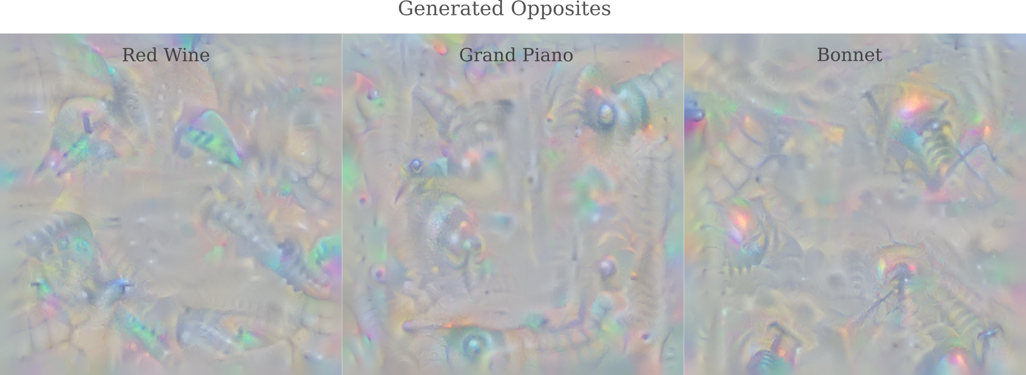
At first consideration, this procedure might not seem to be likely to yield any meaningful input $a_n$, as there is no guarantee that moving away from some class would not yield an input that is a mix of many different objects. And indeed many generated opposite images are apparently a mix of a number of objects, for example this ‘Piano’ opposite that appears to be the image of a few different insects, or the opposite of ‘Bonnet’ that appears to be a mousetrap spring on fire.

Despite it being unlikely that any of the 1000 ImageNet categories would have only one opposite, we can find the category of the image as classified by our model of choice (GoogleNet) by finding which element of the tensor of the model’s output $O(a_n, \theta)$, denoted output, has the maximum activation.

predicted = int(torch.argmax(output))

Now we can label each generated image according to which ImageNet category it most activates using a model of choice, here GoogleNet to be consistent with the image generation. The following video shows the generation of an input $a$ that minimizes the GoogleNet activation for ImageNet class 55: Green Snake (red dot in the scatterplot to the right). Once again, two octaves with Gaussian convolutions are applied during gradient descent.

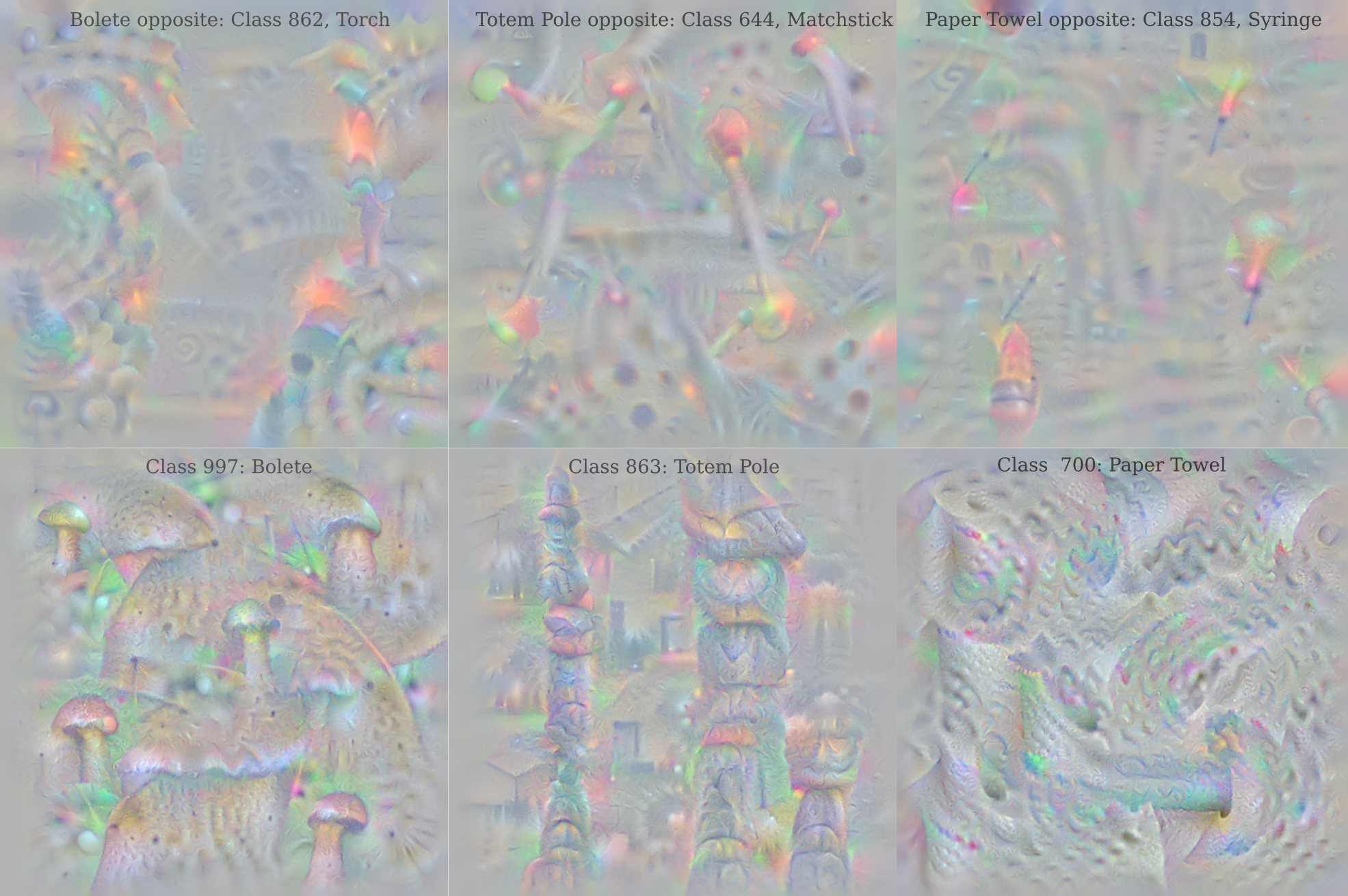
Notice how a number of different categories have been maximized, and how the image appears to be a combination of different parts (an axolotl’s gills with the feet and scales of a crocodile are perhaps the two most obvious). Some objects have more coherent, even reasonable opposites: toilet paper is soft, flat, and waivy whereas syringes are thing and pointy.

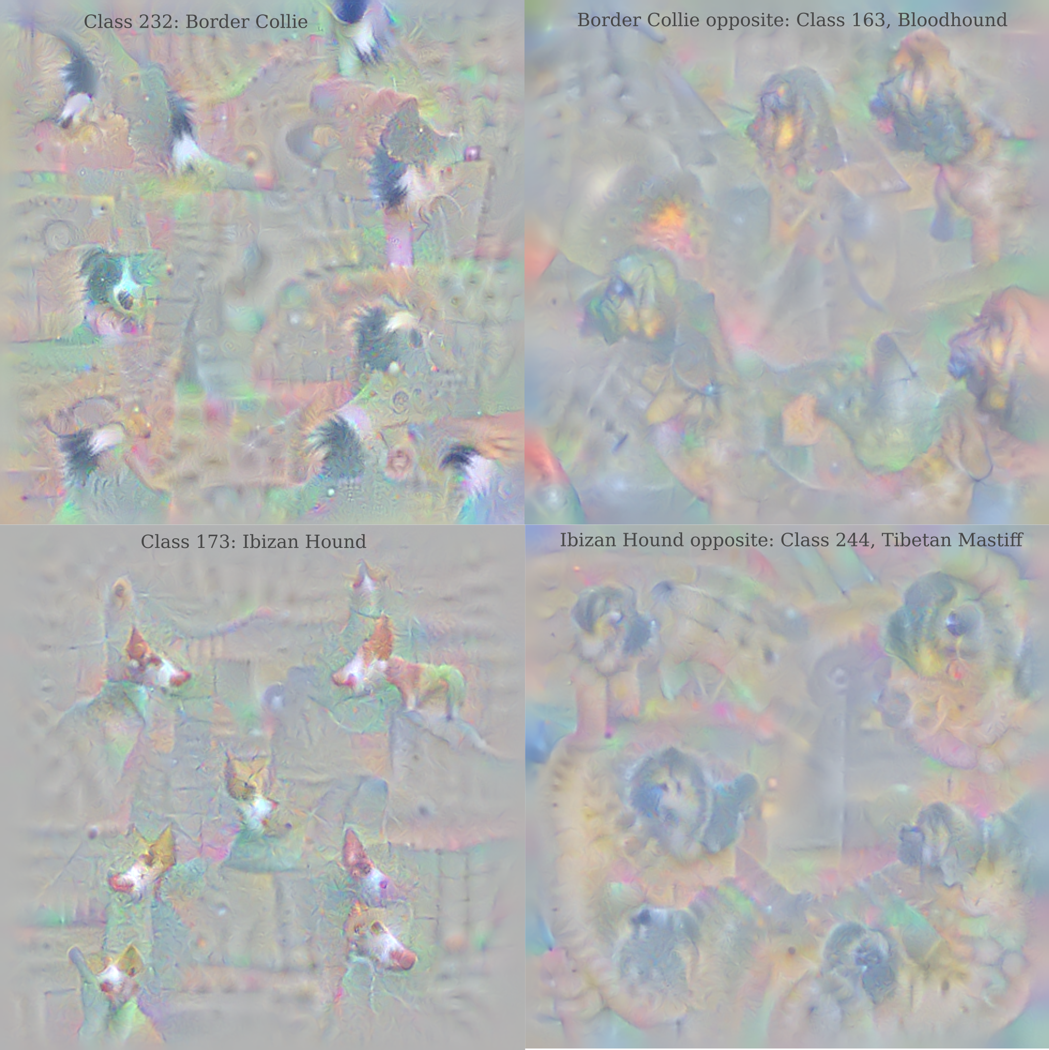
Dogs are perhaps the most interesting image category for this procedure nearly every ImageNet dog class has a coherent opposite that is also a dog, and the opposites generated seem to be logically motivated: observe how the opposites for large, long-haired dogs with no visible ears are small, thin, and perky-eared breeds.

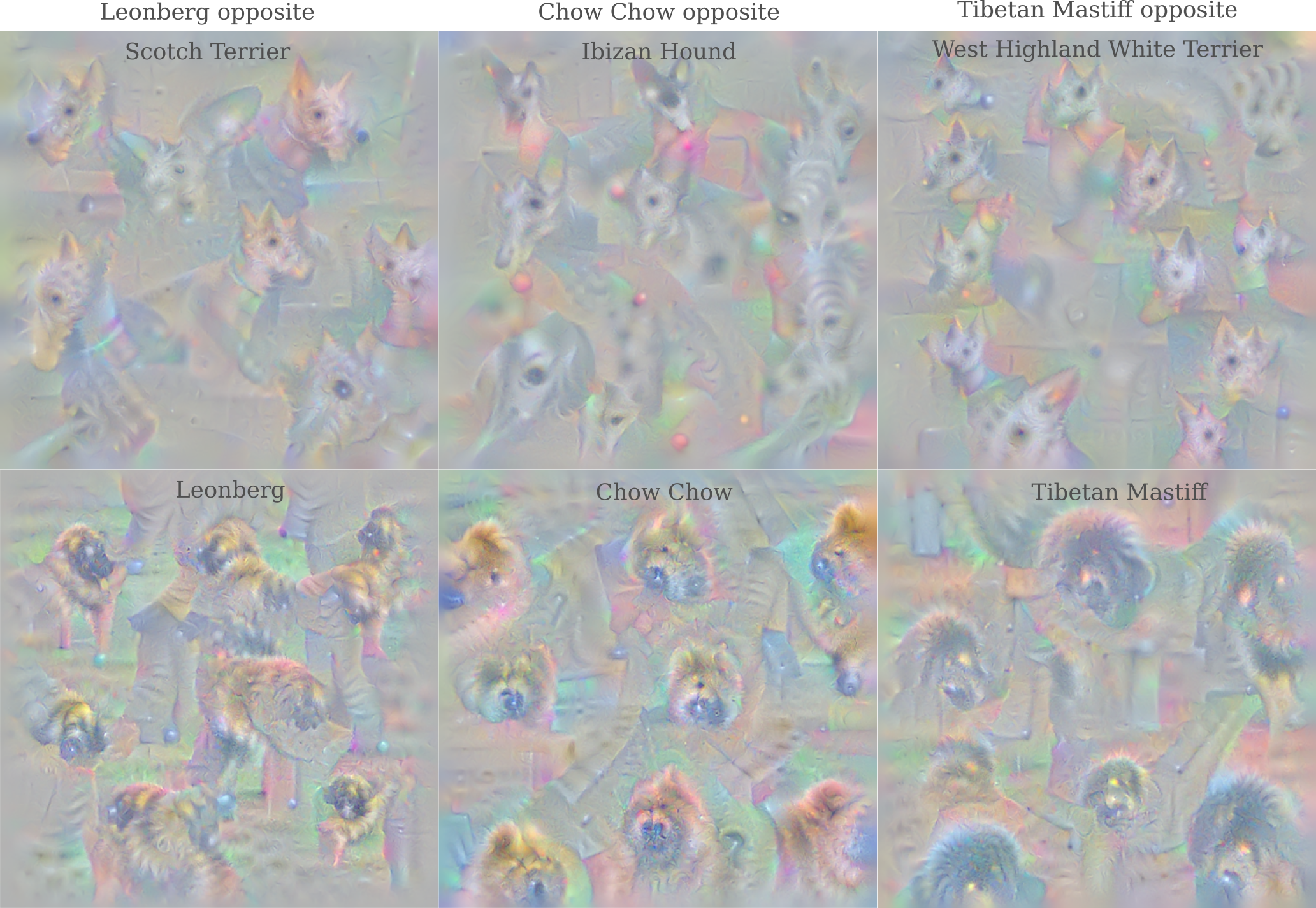
and likewise the opposites of a dog with longer fur and a pointed face (border collie) is one with short fur and squashed face (bloodhound), and the opposite of an image of a small dog with pointed ears (Ibizan hound) is a large dog with droopy ears (Tibetan Mastiff). Observe that opposites are rarely commutative: here we see a close but not quite commutative relation, where the opposite of an Ibizan is a Mastiff but the opposite of a Mastiff is a Terrier. In general opposites are further from being commutative than this example.

It is fascinating to see the generated images for the opposites of other animal classes.

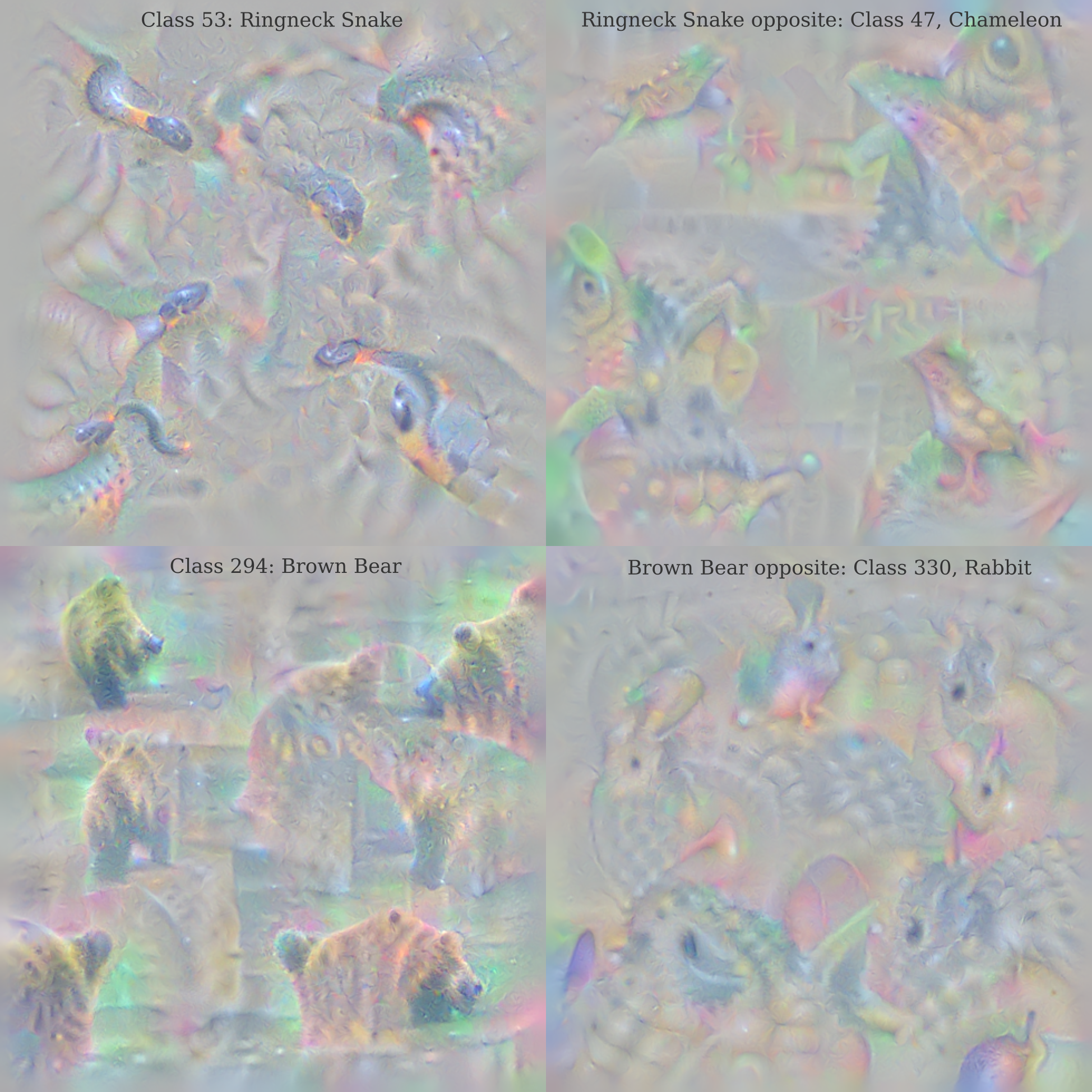
The opposites of snakes are curiously usually lizards (including crocodiles) or amphibians (including axolotls) and the opposites of a number of birds are species of fish. Opposites to all ImageNet class images according to GoogleNet may be found by following this link.

Dog Transfiguration

In the last section, inputs representing the opposites of ImageNet classes were generated using gradient descent such that the gradient used to minimize the activation of the ImageNet class in question $g’$ was $g’ = -g$, i.e. the gradient used to maximize the activation value multiplied by negative one. As the negative value cancels with the gradient descent term $a_{i+1} = a_i - \epsilon * (-g)$ this procedure is sometimes called gradient ascent. Multiplying by negative one is far from the only transformation we can perform, however: here we explore linear combinations of two target classes using InceptionV3, with a real image as a starting point.

We can view the difference between a Husky and a Dalmatian according to some deep learning model by observing what changes as our target class shifts from ‘Husky’ to ‘Dalmatian’, all using a picture of a dalmatian as an input. To do this we need to be able to gradually shift the target from the ‘Husky’ class (which is $\widehat y_{250}$ in ImageNet) to the ‘Dalmatian’ class, corresponding to $\widehat y_{251}$. This can be accomplished by assigning the loss $J_n(0(a, \theta))$ $n=q$ maximum interations, at iteration number $n$ as follows:

\[J_n(O(a, \theta)) \\ = \left(c - \widehat y_{250} * \frac{q-n}{q} \right) + \left(c - \widehat y_{251} * \frac{n}{q} \right)\]

and to the sum on the right we can add an $L^1$ regularizer if desired, applied to either the input directly or the output. Applied to the input, the regularizer is as follows:

\[L_1 (a) = \sum_i \lvert a_i \rvert\]

Using this method, we go from $(\widehat y_{250}, \widehat y_{251}) = (c, 0)$ to $(\widehat y_{250}, \widehat y_{251}) = (0, c)$ as $n \to q$. The intuition behind this approach is that $(\widehat y_{250}, \widehat y_{251}) = (c/2, c/2)$ or any other linear combination of $c$ should provide a mix of characteristics between target classes.

Using InceptionV3 as our model for this experiment, we have we see that this is indeed the case: observe how the fluffy husky tail becomes thin, dark spots form on the fur, and the eye color darkens as $n$ increases.

Vector Addition and Subtraction

We have so far seen that it is possible to generate recognizable images $a’$ that represent the opposites of some original input $a$, where the gradient descent procedure makes the input $a’ = -a$ according to how the model views each input. Likewise it has been observed that linear combinations of the output corresponding to two breeds of dog yield recognizable images where $a’ = ba_0 + ca_1$ for some constant $d$ such that $b + c = d$.

We can explore other vector operations. Vector addition is the process of adding the component vectors in a space, and may be thought of as resulting in a vector that contains some of the qualities of both operands. One way to perform vector addition during gradient descent on the input is to perform each update $a’ = a + \epsilon g$ such that the gradient is

\[g = \nabla_a (C - O_1(a, \theta)) + \nabla_a(C - O_2(a, \theta)) \\ = \nabla_a (2C - O_1(a, \theta) - O_2(a, \theta))\]

which leads to the appearance of merged objects, for example this turtle and snowbird

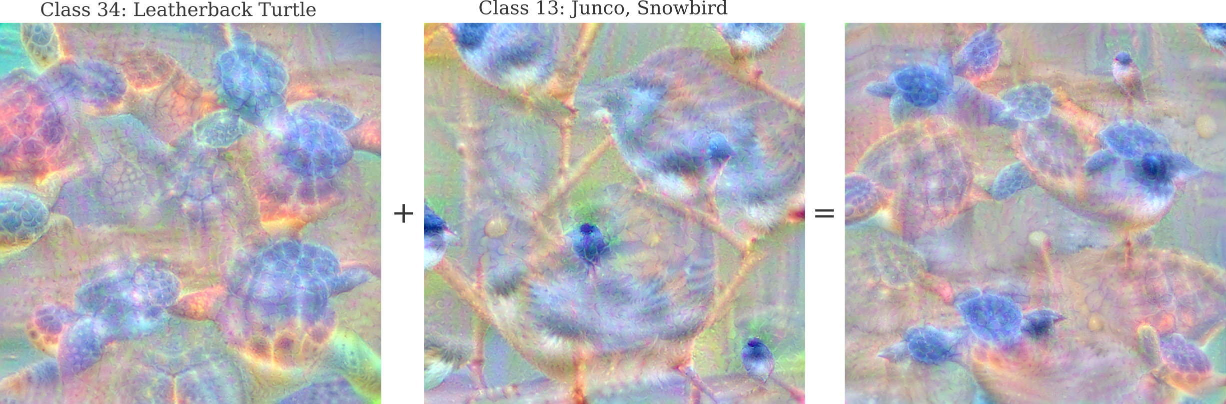
This sort of addition we can call a ‘merging’, as characteristics of both target classes $a_1, a_0$ are found in the same contiguous object. Merging is fairly common using the above gradient.

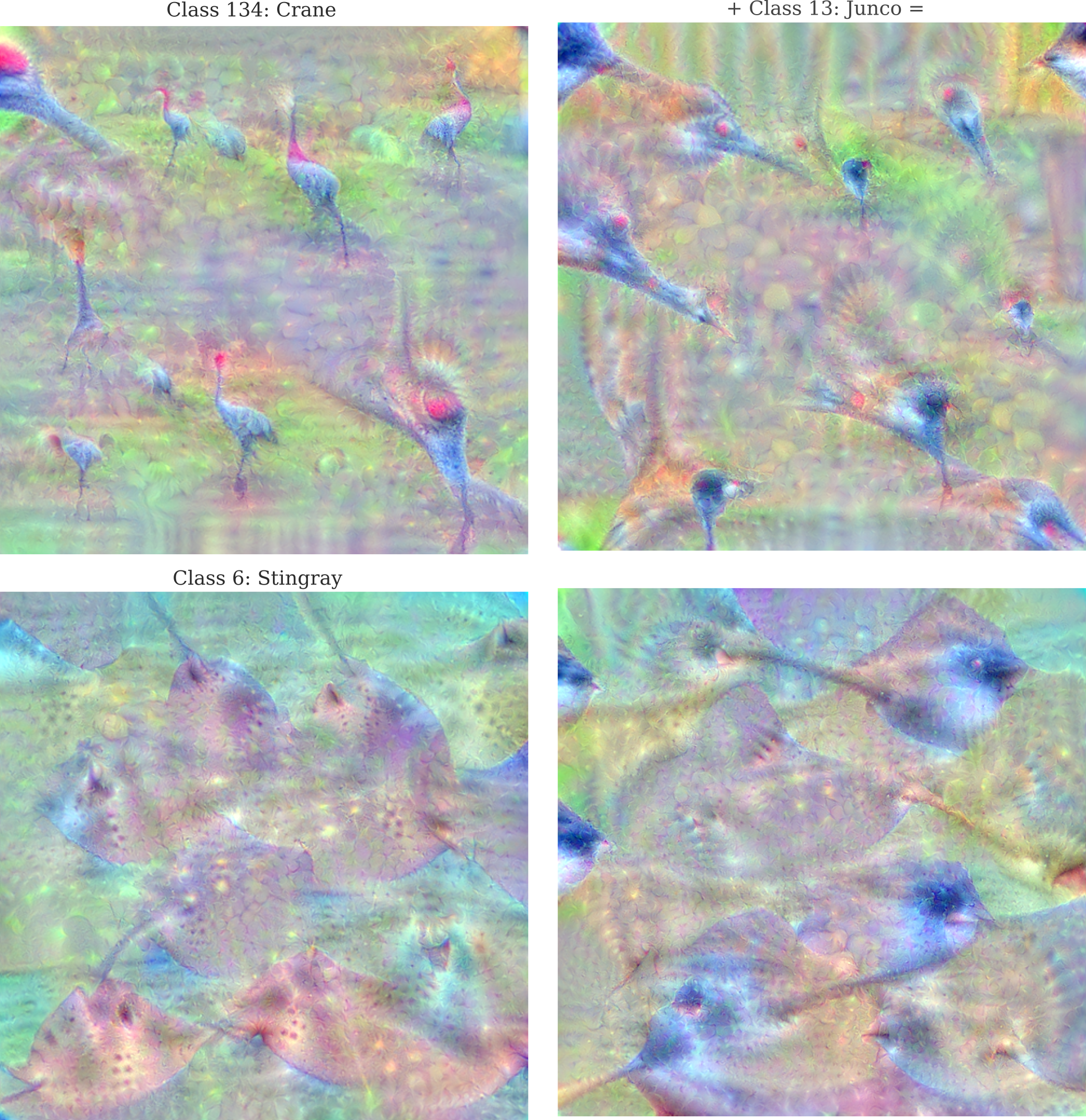
Some target classes tend to make recognizable shapes of one but not both $a_0, a_1$. Instead we can try to optimize the activation of these categories separately, choosing to optimize the least-activated neuron at each iteration. The gradient is therefore

\[g' = \begin{cases} \nabla_a(C - O_2(a, \theta)), & \text{if} \; O_1 \geq O_2 \\ \nabla_a(C - O_1(a, \theta)), & \text{if} \; O_1 < O_2 \end{cases}\]

This $g’$ more often than $g$ when applied to gradient descent does give an image which places both target objects are recognizable and separated in the final image, which we can call juxtaposition.

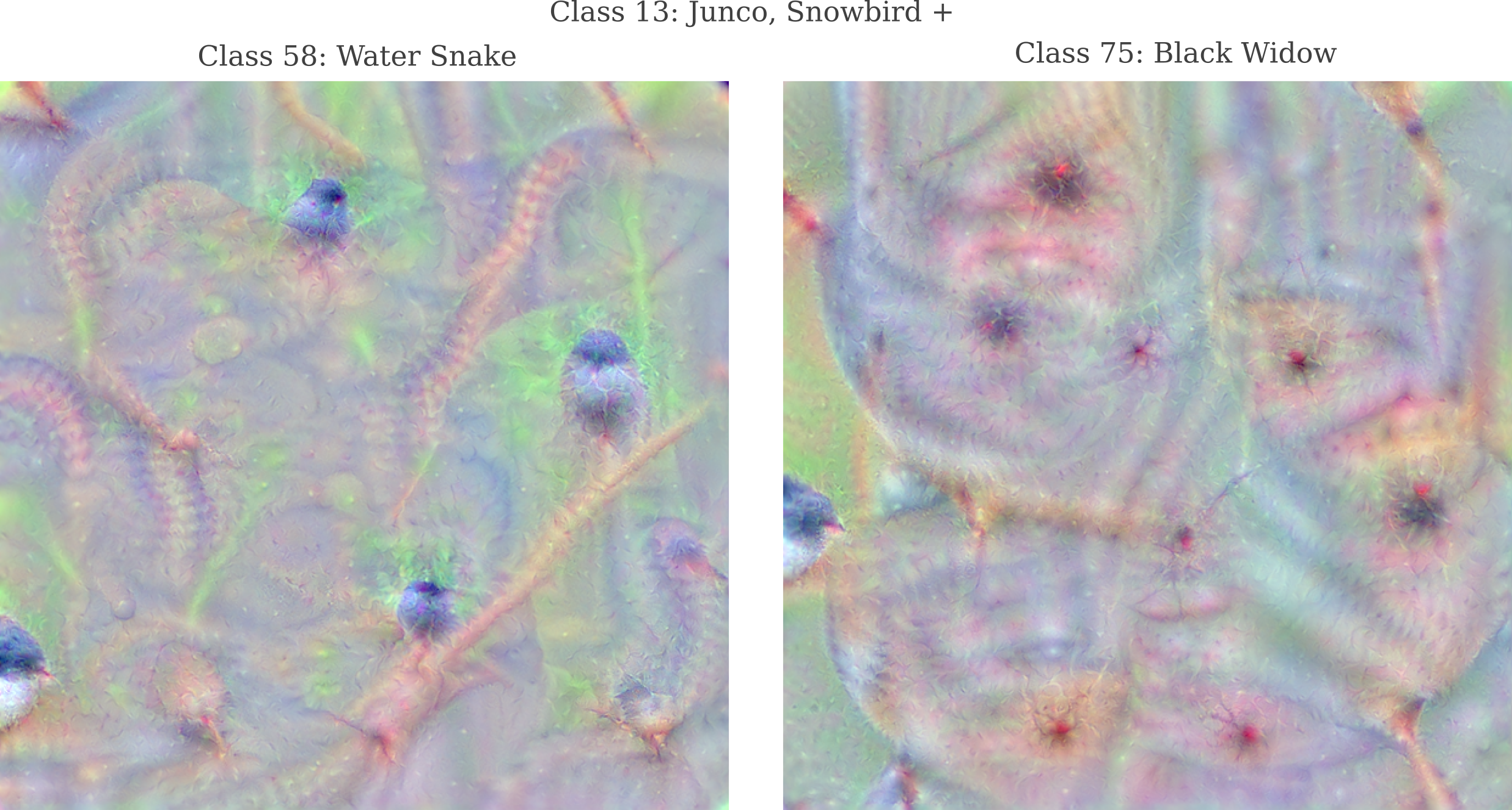
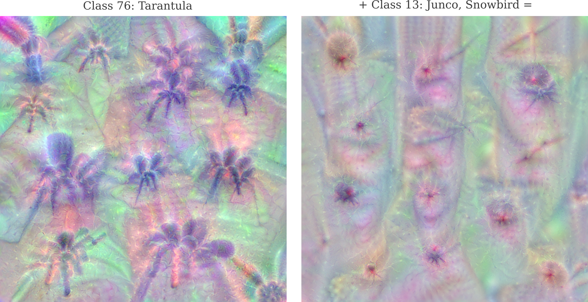
However the addition is performed, there are instances in which the output is neither the merging nor juxtaposition of target class objects. For example, (1) applied to addition of a snowbird to a tarantula yields an indeterminate image somewhat resembling a black widow.

Feature Latent Space

Suppose one were to want to understand which of the ImageNet categories were more or less similar to another. For example, is an image of a cat more similar to a fox or a wolf? Specifically we want this question answered with abstract ideas like facial and tail structure, rather than some simple metric like color alone.

This question is not at all easy to address. We seek a metric that will determine how far ImageNet category is from every other category, but the usual metrics one can place on an image will not be sufficient. Perhaps the simplest way to get this metric is to take the average image for each category (by averaging the values of all images of one category pixel per pixel) and measure the $L^2$ or $L^1$ distance between each image. This is almost certain to fail in our case because there is no guarantee that such a distance would correspond to higher-level characteristics rather than lower-level characteristics like color or hue.

Instead we want a measurement that corresponds to more abstract quantities, like the presence of eyes, number of legs, or roundness of an object in an image. We could use those three traits alone, and make a three-dimensional representation called an embedding consisting of points in space where the basis of the vector space is precisely the values attached to each of these characteristics. For example, if we have some object where [eyes, legs, roundness] = [4, 10, 0.2] we would likely have some kind of insect, whereas the point [-10, -2, 10] would most likely be an inanimate object like a beach ball.

Happily for us, deep learning models are capable of observing high-level characteristics of an image. We have seen that feature maps of certain hidden layers of these models tend to be activated by distinctive patterns, meaning that we can use the total or average activation of a feature map as one of our basis vectors.

Somewhat arbitrarily, let’s choose two features from GoogleNet’s layer 5a as our basis vectors. For reference, here are the maps for the features of interest (meaning that the following images were found to maximally activate the features via gradient descent):

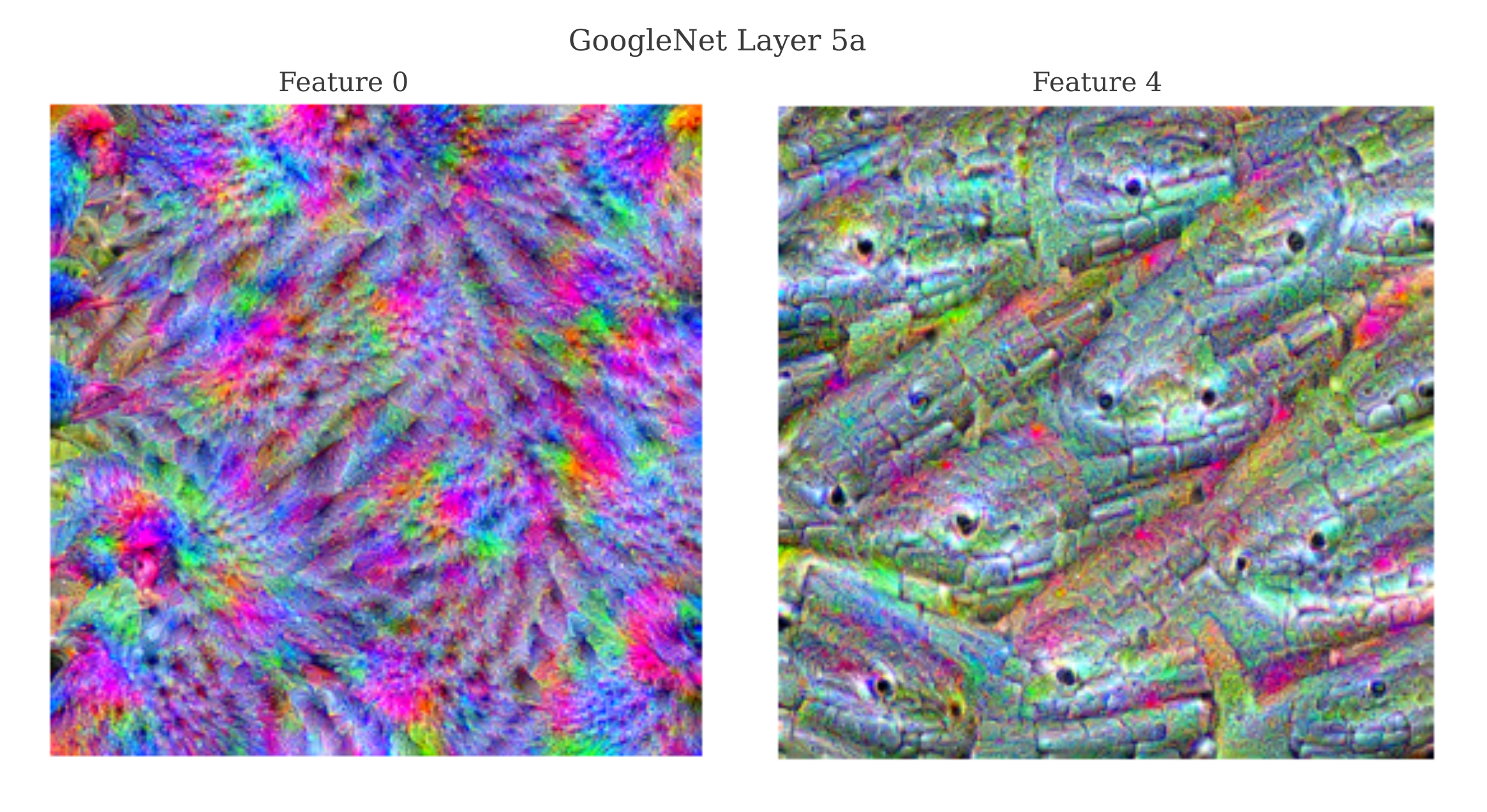
Feature 0 seems to respond to a brightly colored bird-like pattern whereas feature 4 is maximally activated by something resembling a snake’s head and scales. We can observe the activation of these layers for GoogleNet-generated images representing each ImageNet class in order to get an idea of which categories these layers score as more or less similar from each other. The following code allows us to plot the embedding performed by these features by plotting the average activation of the two features for each generated output.

def plot_embedding():
    x, y, labels_arr = [], [], []
    for i, image in enumerate(images):
        label = image[1]
        image = image[0].reshape(1, 3, 299, 299).to(device)
        output = network(image)
        x.append(float(torch.mean(output[0, 0, :, :])))
        y.append(float(torch.mean(output[0, 4, :, :])))
        i = 11
        while label[i] not in ',.':
            i += 1
        labels_arr.append(label[11:i])

    plt.figure(figsize=(18, 18))
    plt.scatter(x, y)
    for i, label in enumerate(labels_arr):
        plt.annotate(label, (x[i], y[i]))
    plt.show()
    plt.close()
    return

this yields

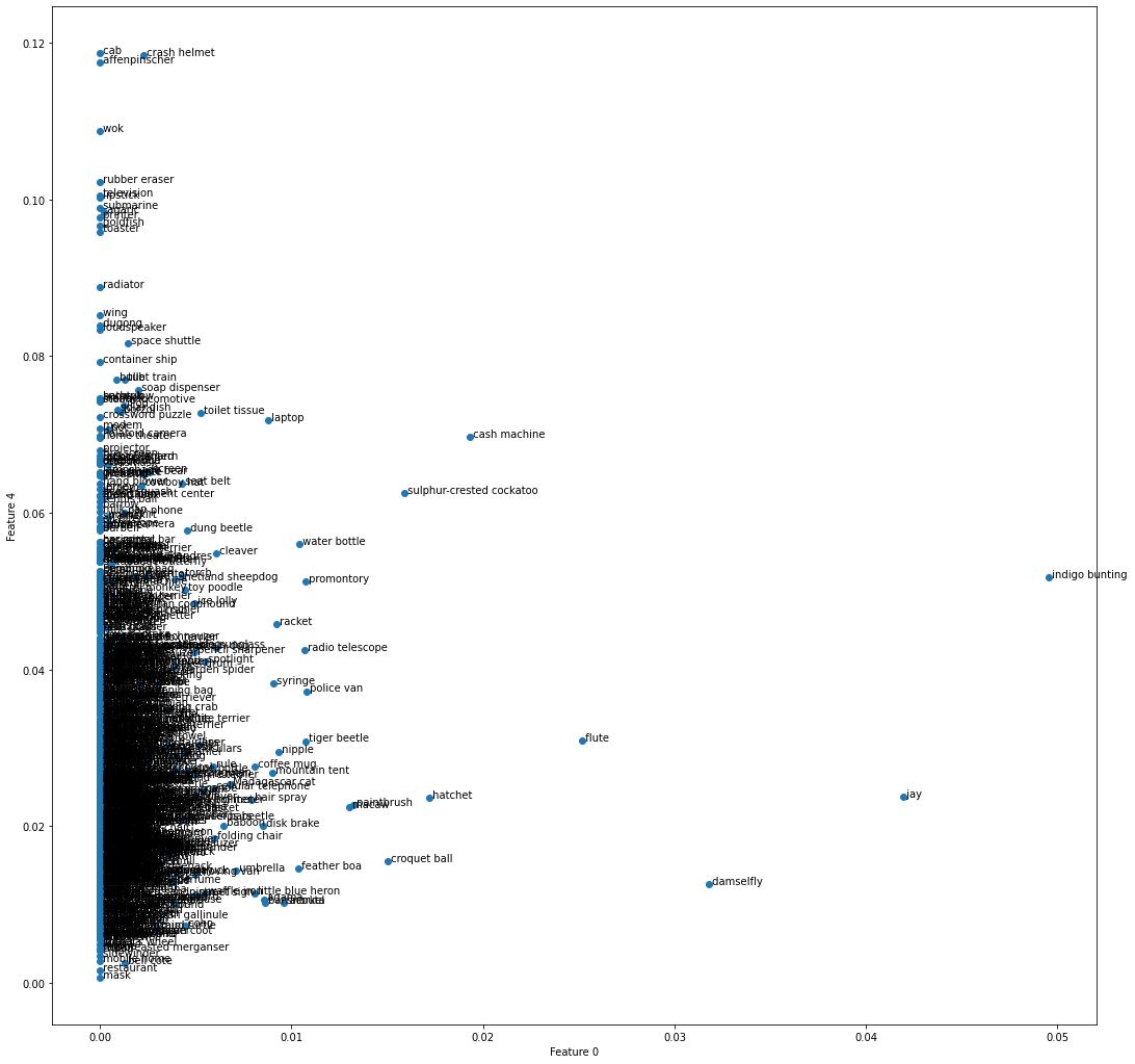
which has noticeably skewed distribution,

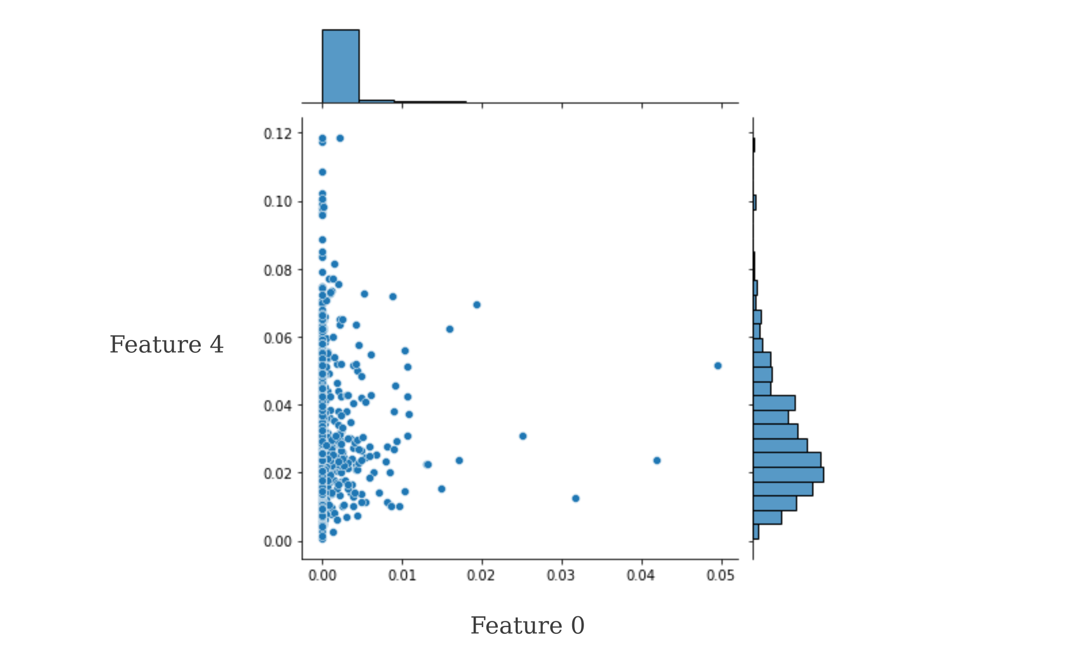
It appears that Feature 0 corresponds to a measure of something similar to ‘brightly-colored bird’ whereas Feature 4 is less clear but is most activated by ImageNet categories that are man-made objects.

Graphs on ImageNet classes

Investigating which ImageNet categories are more or less similar than each other was explored in the previous section using two features from one layer of a chosen model (GoogleNet). But in one sense, these embeddings are of limited use, because they represent only a very small portion of the information that the model possesses in respect to the input images, as there are many more features in that layer and many more layers in the model. To be specific, the embedding diagram in the last section denotes that ‘Jay’ is the ImageNet class most similar to ‘Indigo Bunting’ for GoogleNet, but only for two out of over 700 features of one specific layer.

Each of the features and layers are important to the final classification prediction, and moreover these layers and features are formed by non-linear functions such that the features and layers are non-additive. Therefore although the embeddings of the output categories using feature activation as the basis space is somewhat useful, it is by no means comprehensive. Another approach may be in order in which the entire model is used, rather than a few features.

There does exist a straightforward way to determine which ImageNet categories are more or less similar than each other: we can simply take the model output (with ImageNet classification occuring in the last layer) vector given the generated input $a_g$ which is $y = O(a_g, \theta)$ and observe the magnitudes of the components of this vector. Assuming that the model correctly identifies the generated input, the component of $y$ that is largest will be the target class that $a_g$ was generated to represent. The second-largest component corresponds to a different class that the model considers to be ‘most similar’ to the target class.

There exists a problem with using the this approach as a true similarity metric, however: $y = O(a’, \theta)$ is not guaranteed to be symmetric, or in other words generally $m(a, b) \neq m(b, a)$. This means that we cannot use the findings from the generation metric to make a vector space or any other metric space as the allowable definition of a distance metric is not followed.

But because pairs of points exhibit an asymmetric measurement, we cannot portray this as a metric space. But it is possible to portray these points as an abstract graph, with nodes corresponding to ImageNet categories (ie outputs) and verticies corresponding to relationships between them. We will start by only plotting the ‘nearest neighbor’ relationship, which is defined as the output that is most activated by the generated image distinct from the target output $\widehat y$.

import networkx as nx

def graph_nearest():
    # convert array of pairs of strings to adjacency dict
    closest_dict = {}
    for pair in closest_array:
        if pair[0] in closest_dict:
            closest_dict[pair[0]].append(pair[1])
        else:
            closest_dict[pair[0]] = [pair[1]]

    G = nx.Graph(closest_dict)
    nx.draw_networkx(G, with_labels=True, font_size=12, node_size=200, node_color='skyblue')
    plt.show()
    plt.close()
    return

The first half of the 1000 ImageNet categories are mostly animals, and plotting a graphs for them yields

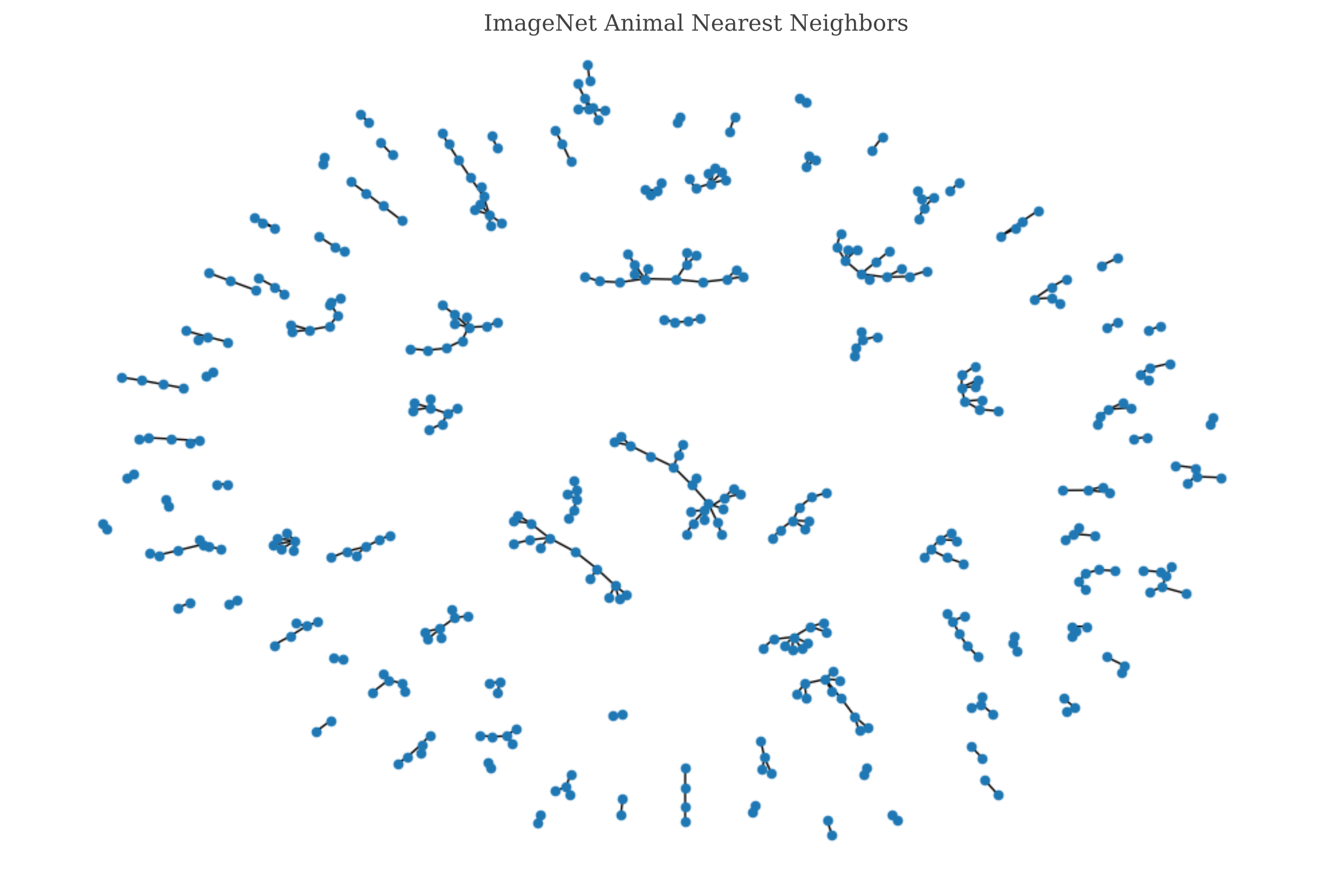
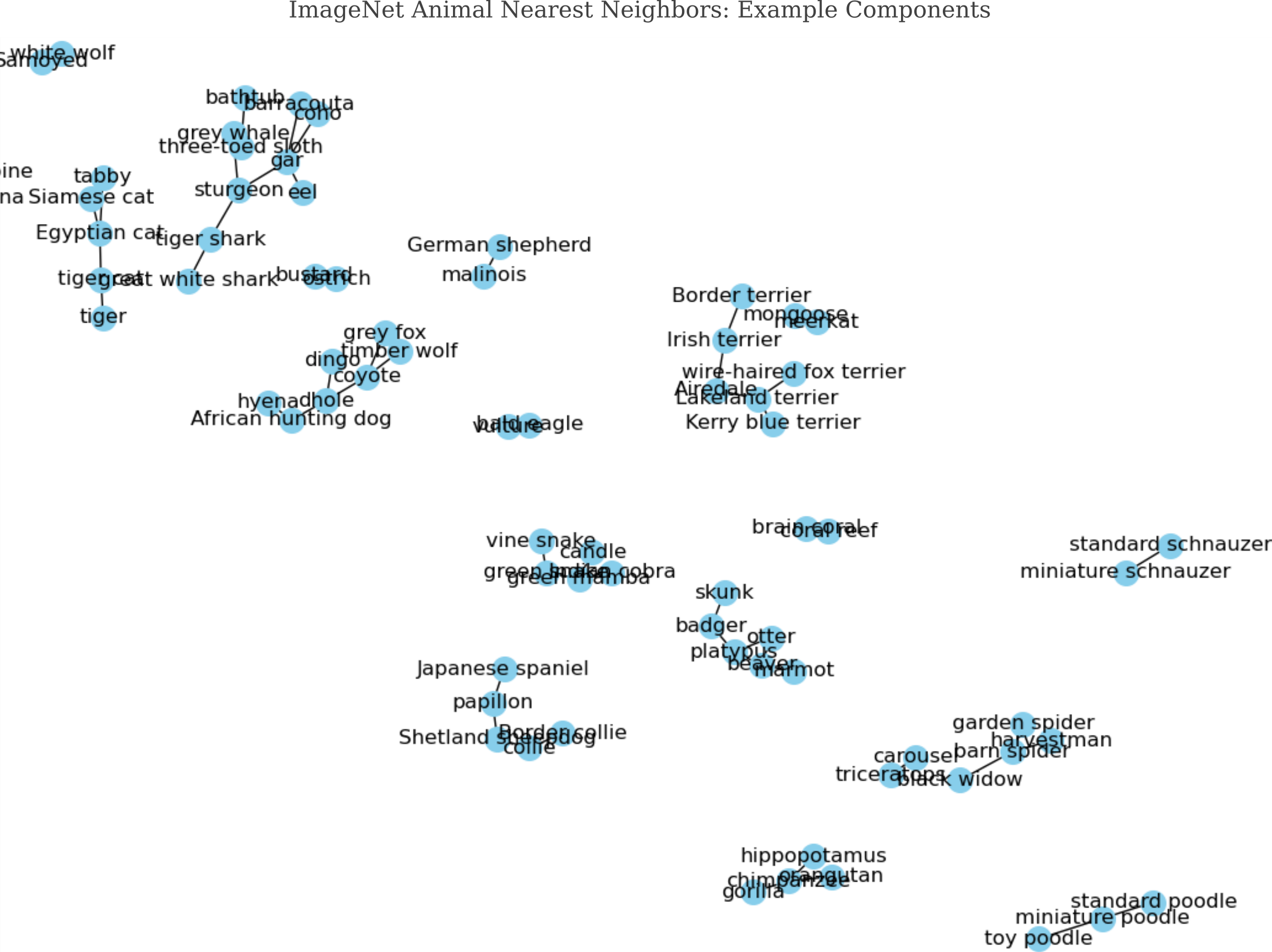
Nodes that are connected together form a ‘component’ of the graph, and nodes that are all connected to each other form a complete component called a ‘clique’. Cliques of more that two nodes are extremely rare for ImageNet nearest neighbors, but non-trivial (ie those with more than two nodes) components abound, often with very interesting and logical structures. Observe how cats form one component, and terrier dogs preside in another, and mustelids and small mammals in another

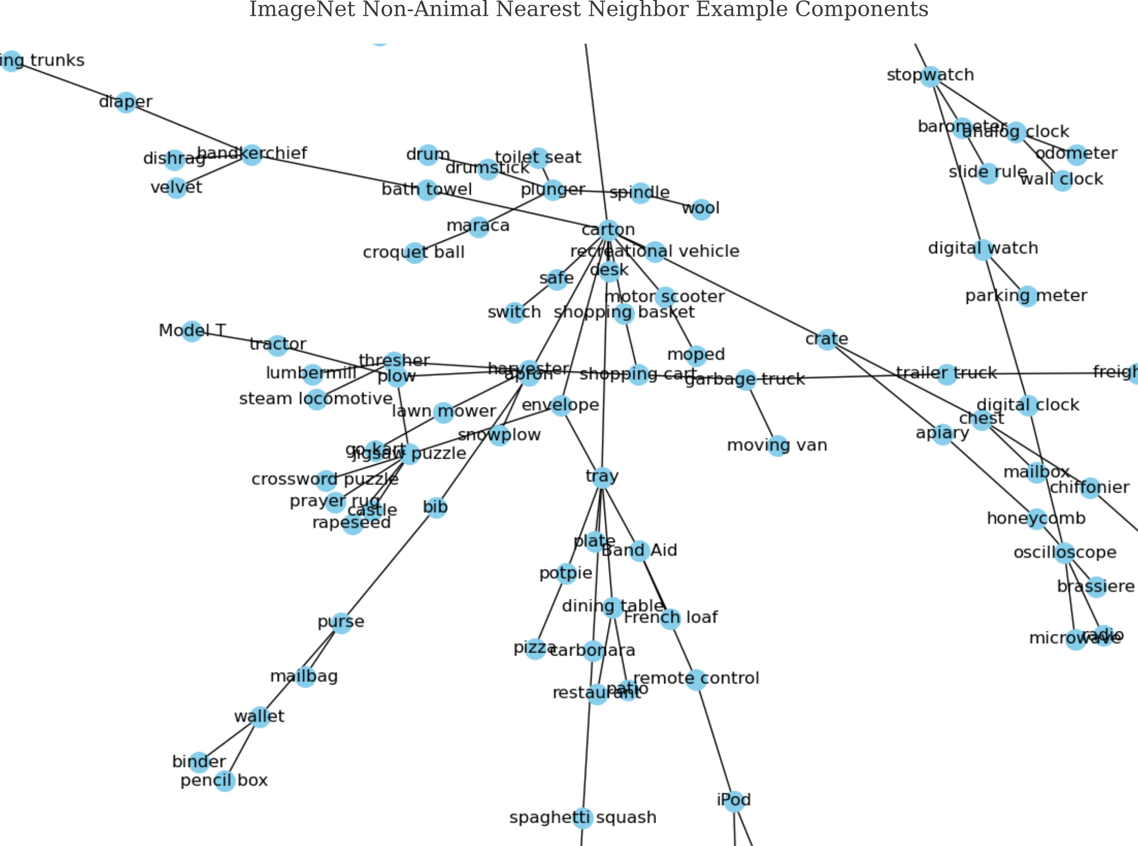
For the non-animal half of ImageNet, graphing nearest neighbors yields a component with more members than was observed for any animal component.

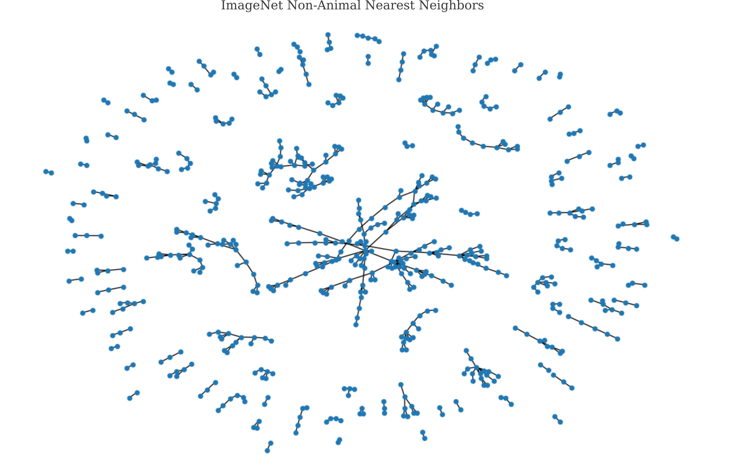
This contains many diverse objects, yet often still exhibit relationships that seem reasonable to a human.

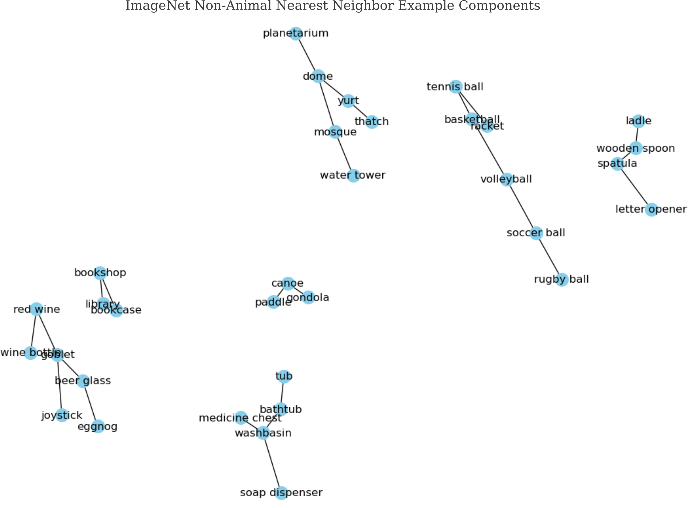
Smaller components are often the most illuminating: observe the sports balls clustering together in one component, and the utensils in another component

Output Latent Space

The above measurement is illuminating but is not a true metric space. Instead of finding the second largest output for our generated inputs, we can find the ImageNet class corresponding to the second closest point (including the point of interest) to our point in the output space. This means that we wish to perform an embedding of the output with respect to the model. The reasoning here is that our trained GoogleNet model with parameters $\theta$ may be viewed as a (very complicated) function $O$ that maps input images $a$ to an output $y$, which is a 1000-dimensional vector where the element of index $n$ denoted by $y_n$.

\[y = O(a, \theta)\]

Now if we use real images from some category, there is no guarantee that $v$ will be unchanged and it is unclear which $v$ best respresents the image category. Instead we can use an image $a’$ generated to maximize the output category of interest (for more information on this, see here) as an approximation of the input that will most resemble the output category of interest $\widehat y_n = O_n(a, \theta)$.

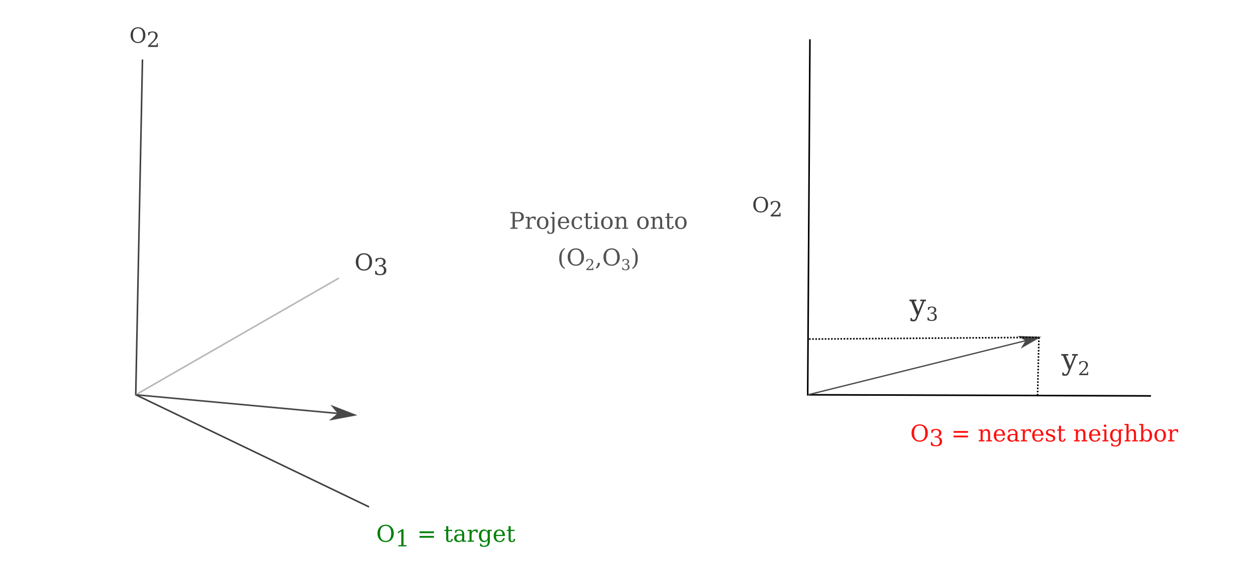
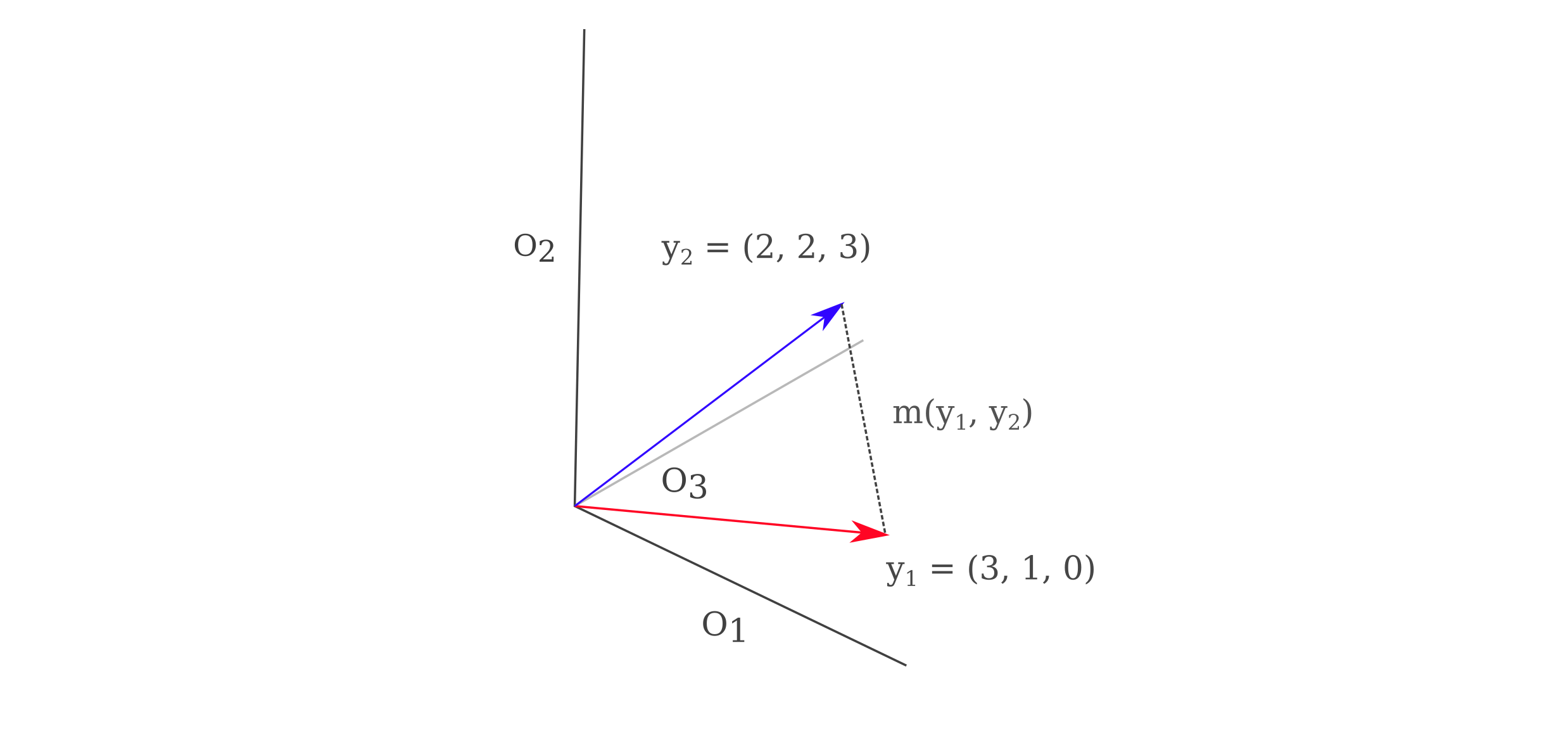
\[a' = \mathrm{arg} \; \underset{a}{\mathrm{max}} \; O_n(a, \theta)\]

Using these representative inputs $a’$ applied to $O$, we can find the coordinates of all model outputs $y_n \in \Bbb R^{1000}$. This means that we can find the coordinates of the representative input $a’$ in the 1000-dimensional output space. For a three-dimensional example of this method see the following figure. Note that the metric $m(y_1, y_2)$ may be chosen from any number of possible methods.

As spaces with more than two or three dimensions are hard to visualize, we can perform a dimensionality reduction method for visualization, and here we will find a function $f$ to take $f: y_n \in \Bbb R^{1000} \to z_n \in \Bbb R^2$. We shall employ principle component analysis, which is defined as the function $f(y)$ that produces the embedding $z$ such that a decoding function $g$ such that $x \approx g(f(y))$, where $g(y) = Dy$ and $D \in \Bbb R^{1000x2}$. Therefore PCA is defined as the encoding function $f$ that minimized the distance of the encoded value $z$ from the original value $y$ subjected to the constraint that the decoding process be a matrix multiplication. To further simplify things, $D$ is constrained to have linearly independent columns of unit norm. The minimization procedure may be accomplished using eigendecomposition and does not requre gradient descent.

When we find the coordinates of $y_n$ for all $n$ ImageNet categories using GoogleNet and then map these points using the first two principle components

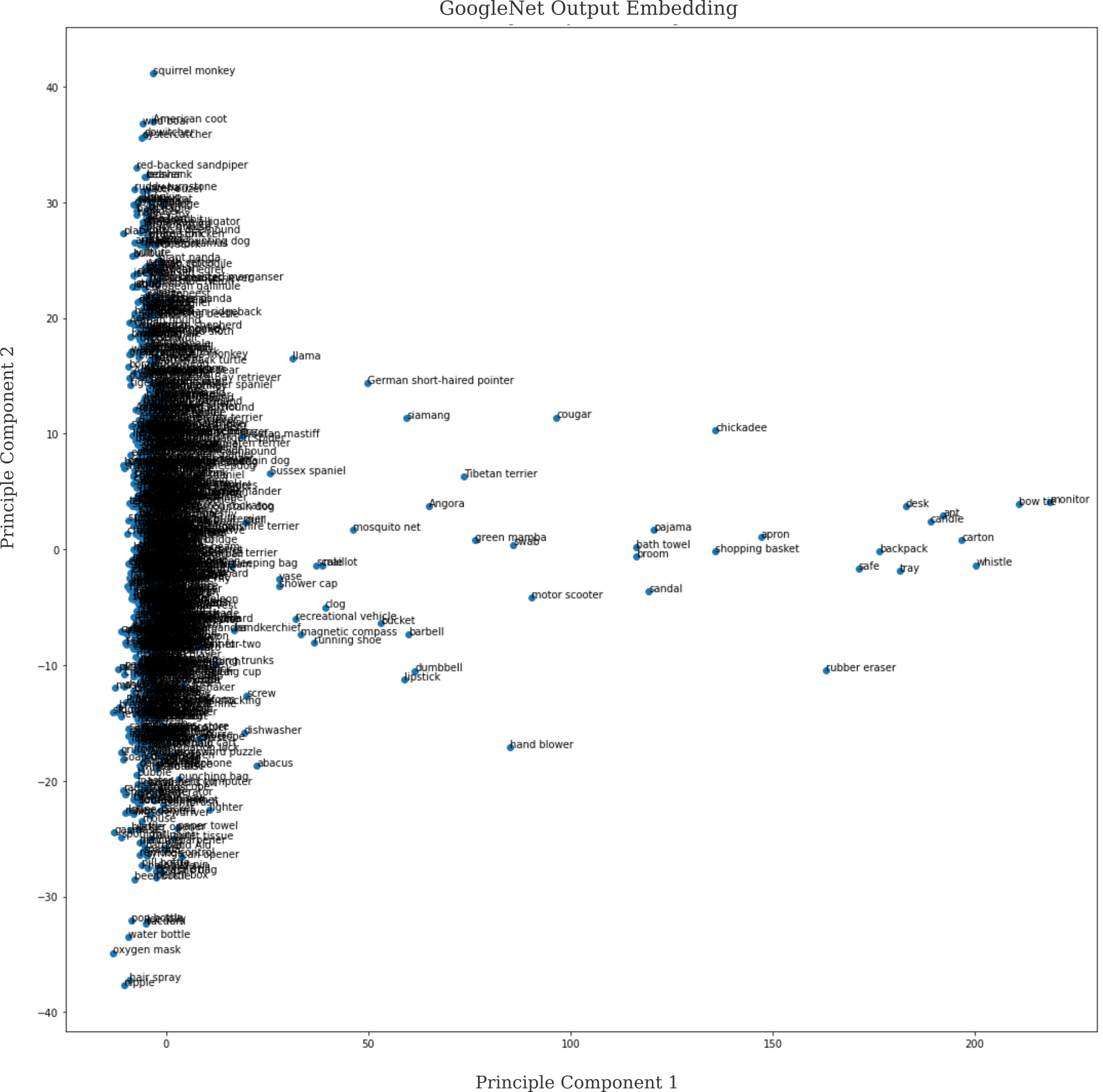
but the result is somewhat underwhelming. Principle conponents 1 and 2 account for only $15$ and $4$ percent (respectively) of the variance, meaning that they capture very little of the original distribution.

Why is this the case? The failure lies in PCA’s expectation of a linear space, in which transformations $f$ are additive and scaling

\[af(x + y) = f(ax) + f(ay)\]

and where in particular the intuitive metric of distance stands. As points in this space were generated using a nonlinear function (gradient descent of GoogleNet on a scaled normal input), there is no reason to think that a linear decomposition would be capable of capturing much of the variance in that function.