Image Generation with Classification Models I
Modifying an input via gradient descent
The observation that a deep learning model may be able to capture much of the inportant information in the input image leads to a hypothesis: perhaps we could use a trained model in reverse to generate inputs that resemble the training inputs.
On this page we saw that the loss gradient with respect to the input $\nabla_a J(O(a; \theta), y)$ of a trained model is able to capture certain features of input images: in particular, the gradient mirrors edges and certain colors that exist in the input. This observation leads to an idea: perhaps we could use this gradient to try to make our own input image by starting with some known distribution and repeatedly applying the loss gradient to the input. This process mirrors how stochastic gradient descent applies the loss gradient with respect to the model parameters each minibatch step, but instead of modifying the model parameters instead we are going to modify the input itself.
If we want to apply the loss gradient (of the input) to the input, we need three things: a trained model with parameters $\theta$, and input $a$, and an output $y$. One can assign various distributions to be the input $a$, and arbitrarily we can begin with a stochastic distribution rather than a uniform one. Next we need an output $y$ that will determine our loss function value: the close the input $a$ becomes to a target input $a’$ that the model expects from learning a dataset given some output $y$, the smaller the loss value. We can also arbitrarily choose an expected output $\widehat{y}$ with which we use to modify the input, but for a categorical image task it may be best to choose one image label as our target output $\widehat{y}$
Each step of this process, the current input $a_n$ is modified to become $a_{n+1}$ as follows
\[a_{n+1} = a_n - \epsilon \nabla_a J(O(a; \theta), \widehat{y})\]Intuitively, a trained model should know what a given output category generally ‘looks like’, and performing gradient-based updates on an image while keeping the output constant (as a given category) is similar to the model instructing the input as to what it should become to match the model’s expectation.
To implement this algorithm, first we need a function that can calculate the gradient of the loss function with respect to the input
def loss_gradient(model, input_tensor, true_output, output_dim):
	...
	true_output = true_output.reshape(1)
	input_tensor.requires_grad = True
	output = model.forward(input_tensor)
	loss = loss_fn(output, true_output) # loss applied to y_hat and y

	# backpropegate output gradient to input
	loss.backward(retain_graph=True)
	gradient = input_tensor.grad
	return gradient
Then the gradient update can be made at each step
def generate_input(model, input_tensors, output_tensors, index, count):
	...
	target_input = input_tensors[index].reshape(1, 3, 256, 256)
	single_input = target_input.clone()
	single_input = torch.rand(1, 3, 256, 256) # uniform distribution initialization

	for i in range(1000):
		single_input = single_input.detach() # remove the gradient for the input (if present)
		predicted_output = output_tensors[index].argmax(0)
		input_grad = loss_gradient(model, single_input, predicted_output, 5) # compute the input gradient
		single_input = single_input - 10000*input_grad # gradient descent step
single_input can then be viewed with the target label denoted
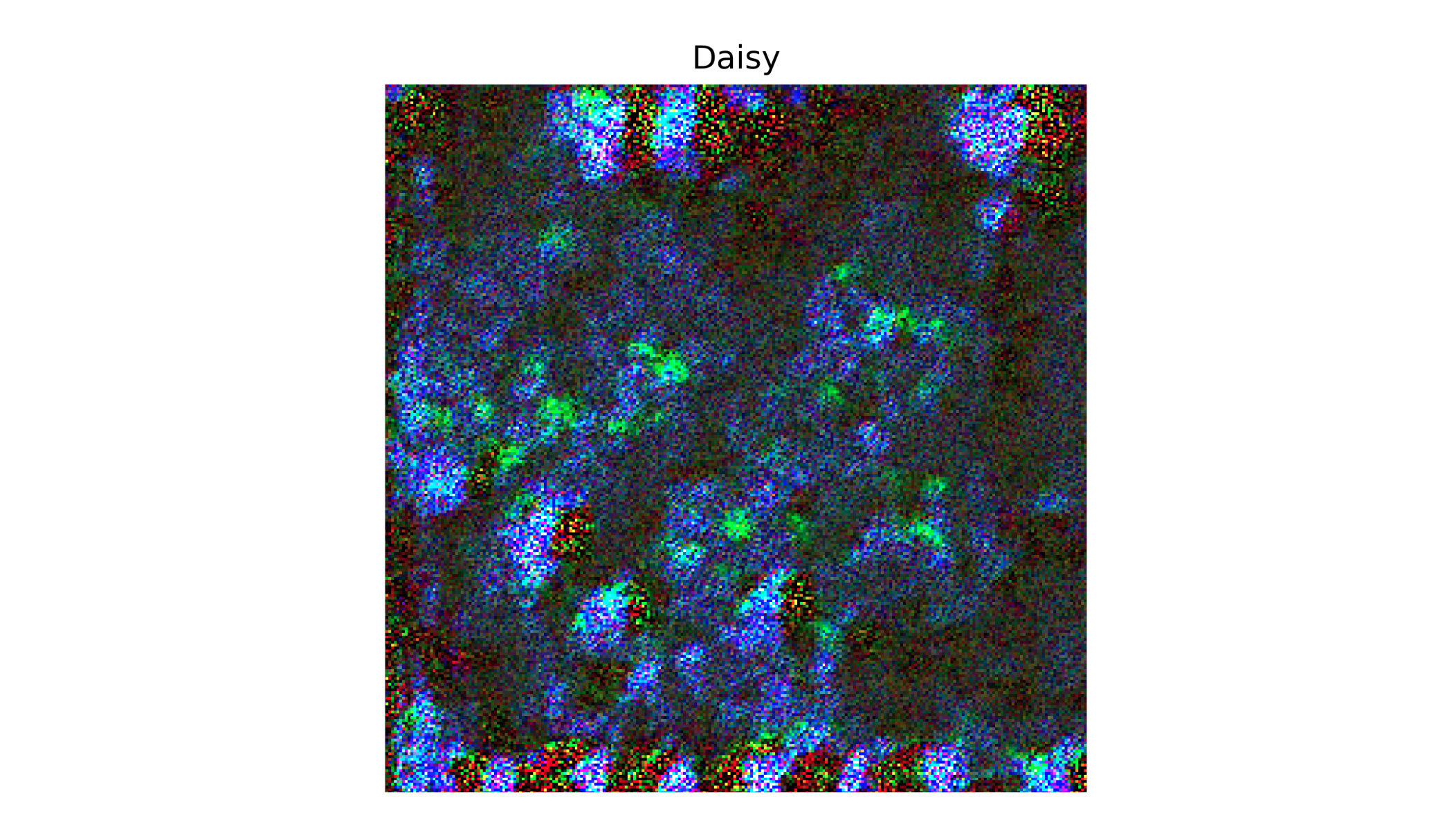
but the output does not really look like a daisy, or a field of daisies.
There are a few challenges using this approach. Firstly, in general many iterations are required such that updating the input may take a good deal of computational power, and furthermore it may be difficult to predict how large to make $\epsilon$ without prior experimentation.
The second problem is that in general there are discontinuities present in the mathematical function describing the mapping of an input $a$ to the output loss $J(O(a; \theta))$ which necessarily makes the reverse function from output to input also discontinuous. We are not strictly using the inverse of forward propegation but instead use the gradient of this loss function to generate the input, but if $J(O(a; \theta))$ is discontinuous then so will its gradients be too.
It has been hypothesized that adversarial examples exist in spite of the high accuracy achieved various test datasets because they are very low-probability inputs. In some respects this is true, as the addition of a small vector in a random direction (rather than the direction of the gradient with respect to the output) very rarely changes the model’s output.
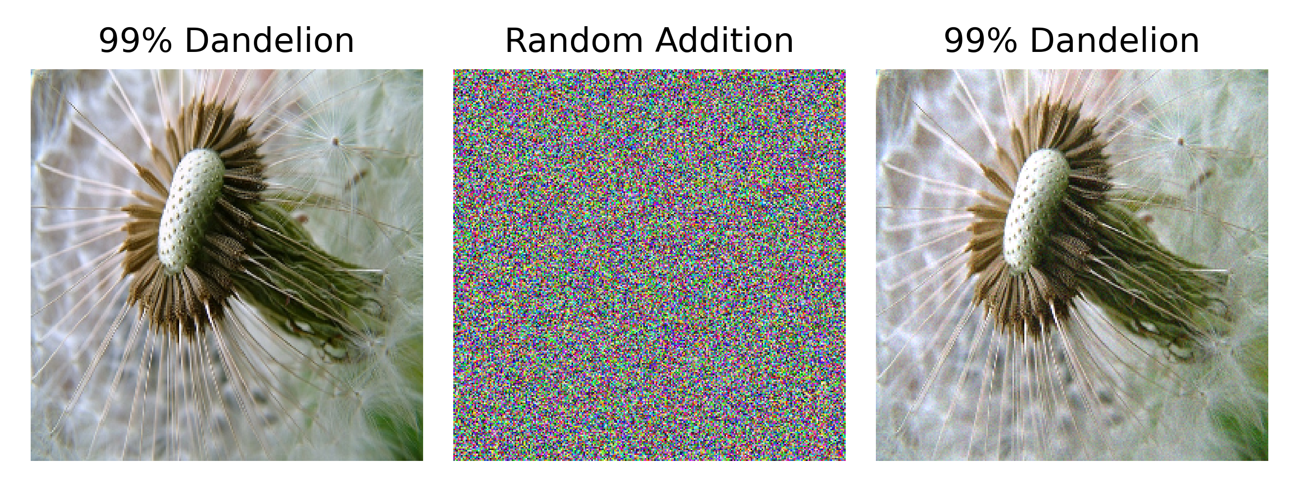
But this is only the case when we look at images that are approximations of inputs that the model might see in a training or test set. In the adversarial example approaches taken on this page, small shifts are made to each element (pixel) of a real image to make an approximately real image. If we no longer restrict ourselves in this way, we will see that adversarial examples are actually much more common. Indeed that almost any input that a standard image classification model would classify as any given label with high confidence does not resemble a real image. For more information on this topic, see the next section.
In practice the second problem is more difficult to deal with than the first, which can be overcome with clever scaling and normalization of the gradient. The main challenge for input generation is therefore that the gradient of the loss (or the output, for that matter) with respect to the input $a$, $\nabla_a J(O(a, \theta))$ is approximately discontinuous in certain directions, which can cause a drop in the loss even though the input is far from a realistic image. The result is that more or less unrecognizable images like the one above are confidently but erroneously classified as being an example of the correct label. For more on the topic of confident but erroneous classification using deep learning, see this paper.
One way to ameliorate these problems is to go back to our gradient sign method rather than to use the actual gradient. This introduces the prior assumption that This allows us to restrict the changes at each iteration to a constant step, stabilizing the gradient update.
\[a_{n+1} = a_n - \epsilon \; \mathrm {sign} \; (\nabla_a J(O(a; \theta), \widehat{y}))\]which for $\epsilon=0.01$ can be implemented as
	...
	for i in range(100):
		single_input = single_input.detach() # remove the gradient for the input (if present)
		# predicted_output = output_tensors[index].argmax(0)
		input_grad = loss_gradient(model, single_input, target_output, 5) # compute input gradient
		single_input = single_input - 0.01*torch.sign(input_grad) # gradient descent step
Secondly, instead of starting with a random input we can instead start with some given flower image from the dataset. The motivation behind this is to note that the model has been trained to discriminate between images of flowers, not recognize images of flowers compared to all possible images in $\Bbb R^n$ with $n$ being the dimension of the input.
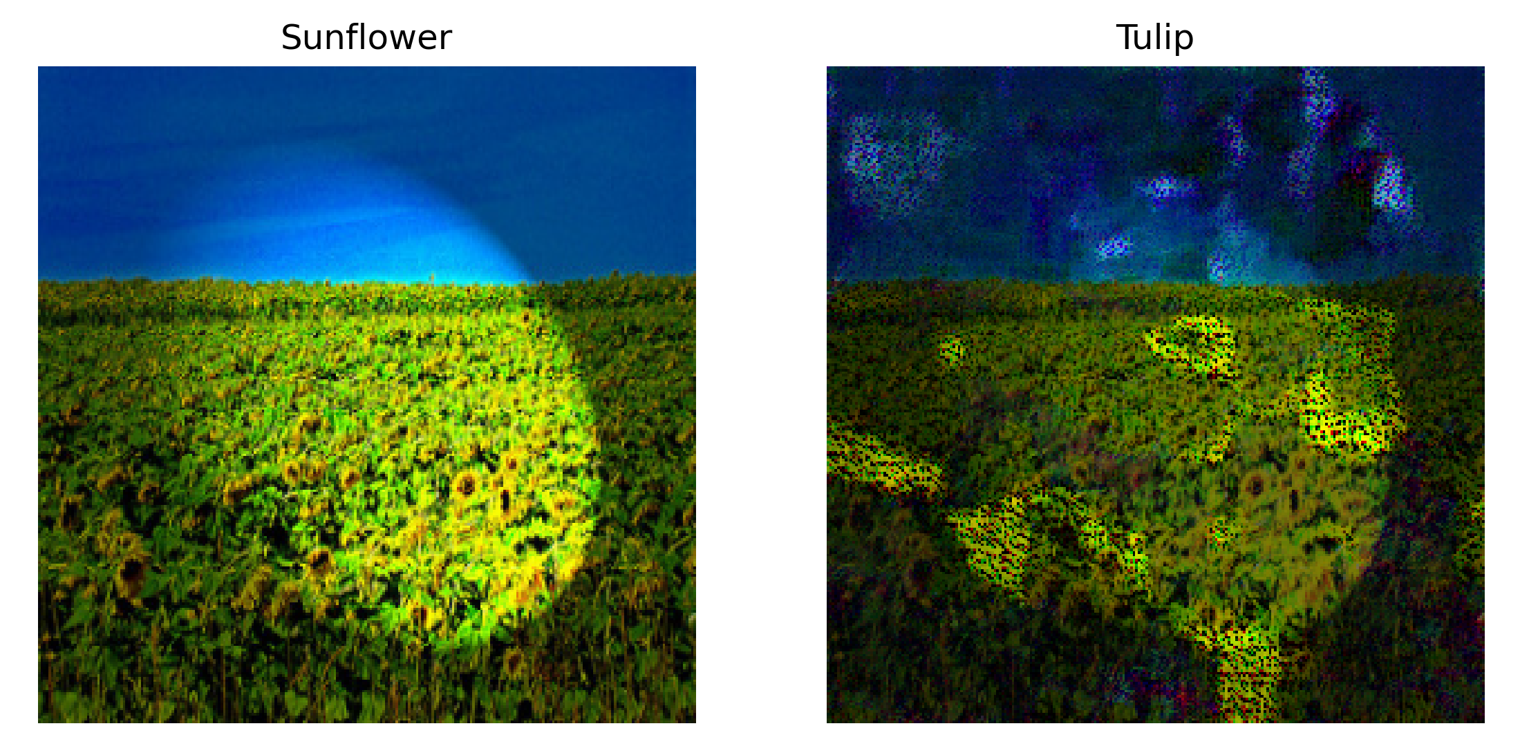
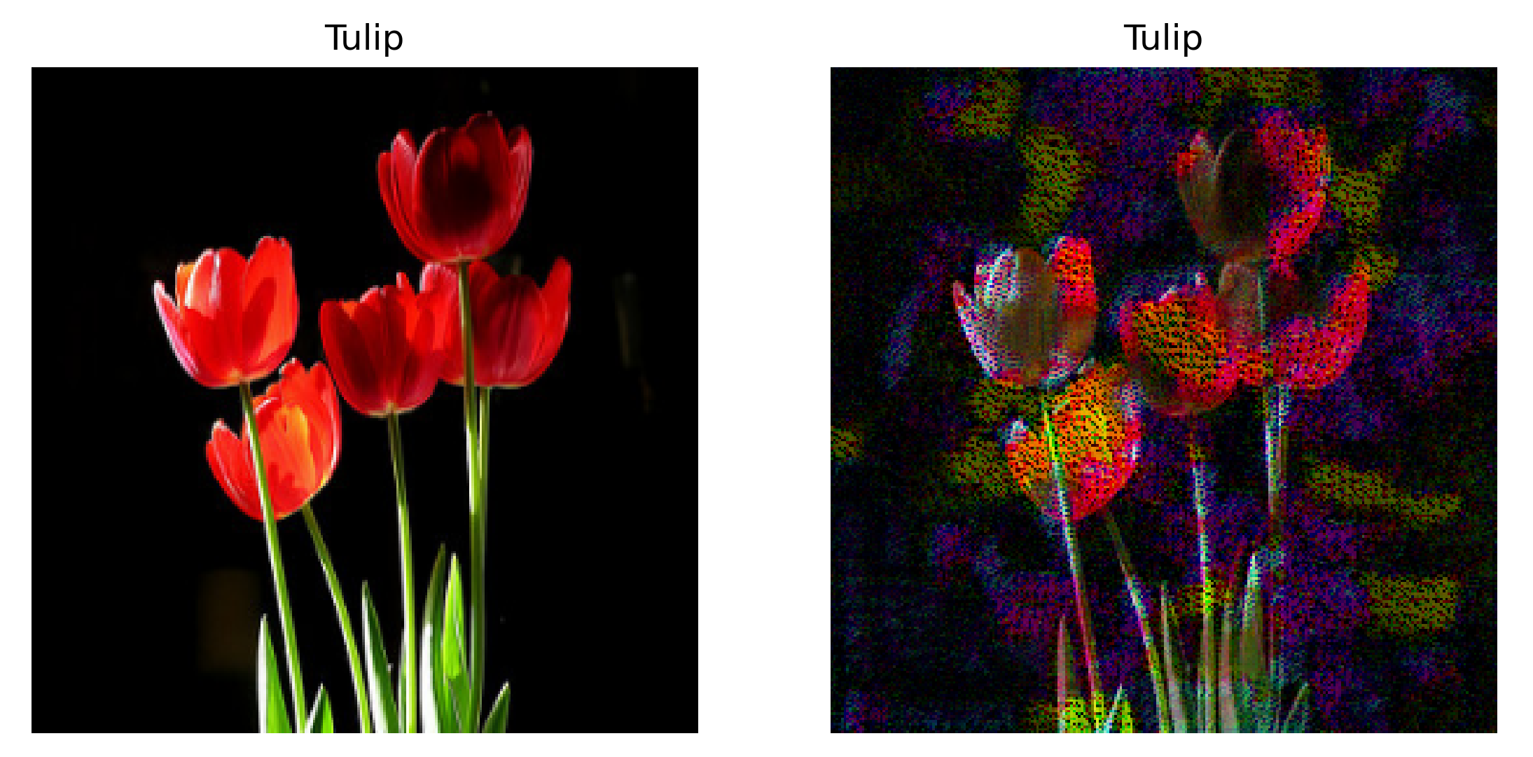
This method is more successful: when the target label is a tulip, observe how a base and stalk is added to a light region of an image of a field of sunflowers,
and how an image of a daisy and a rock is modified to appear more like a field of tulips,
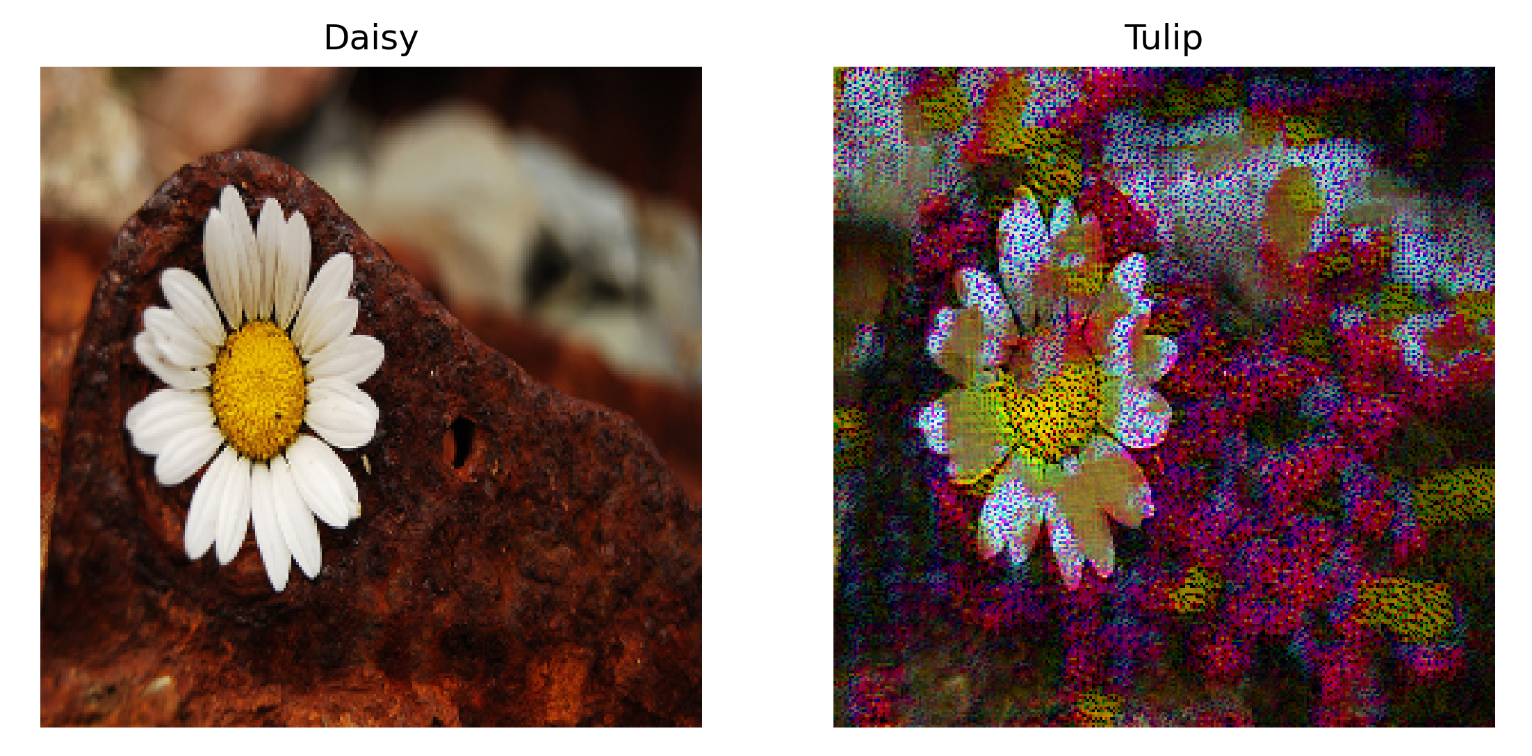
but generally images of tulips are changed less, which is to be expected given that the gradient of the loss function with respect to the input will be smaller if our target output matches our actual output.
Generating Images using a Smoothness Prior
In the last section we saw that using the gradient of the output with respect to the input $\nabla_a J(O(a, \theta))$ may be used to modify the input in order to make it more like what the model expects a given parameter label to be. But applying this gradient to an initial input of pure noise was not found to give a realistic representation of the desired type fo flower, because the loss function is discontinuous with respect to the input. Instead we find a type of adversarial example which is confidently assigned to the correct label by the model, but does not actually resemble any kind of flower at all.
Is there some way we can prevent our trained deep learning models from making unrealistic images during gradient descent on a random input? Research into this question has found that indeed there is a way: restrict the image modification process such that some quality of a real image is enforced. We will proceed with this investigation using an Inceptionv3 (aka GoogleNetv3) trained on the full ImageNet dataset, which consists of labelled images of 1000 classes.
The inception architecture was designed to allow for deeper networks without an exorbitant increase in the number of parameters used. InceptionV3 (as published here) has the following architecture:
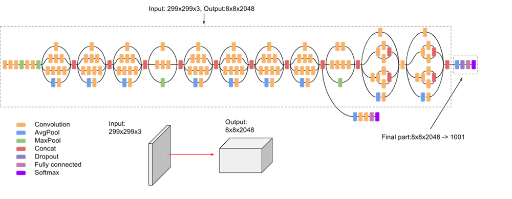
(image source: Google docs)
After loading the model with model = torch.hub.load('pytorch/vision:v0.10.0', 'inception_v3', pretrained=True).to(device), we can use the following function
def count_parameters(model):
	table = PrettyTable(['Modules', 'Parameters'])
	total_params = 0
	for name, parameter in model.named_parameters():
		if not parameter.requires_grad:
			continue
		param = parameter.numel()
		table.add_row([name, param])
		total_params += param
	print (table)
	print (f'Total trainable parameters: {total_params}')
	return total_params
to find that this is a fairly large model with 27161264, or just over 27 million, trainable parameters.
+--------------------------------------+------------+
|               Modules                | Parameters |
+--------------------------------------+------------+
|      Conv2d_1a_3x3.conv.weight       |    864     |
|       Conv2d_1a_3x3.bn.weight        |     32     |
|        Conv2d_1a_3x3.bn.bias         |     32     |
|      Conv2d_2a_3x3.conv.weight       |    9216    |
|       Conv2d_2a_3x3.bn.weight        |     32     |
|        Conv2d_2a_3x3.bn.bias         |     32     |
... (shortened for brevity)...
|              fc.weight               |  2048000   |
|               fc.bias                |    1000    |
+--------------------------------------+------------+
Now that we have our trained model, which qualities of a real image should be enforced during gradient descent? A good paper on this topic by Olah and colleages details how different research groups have attempted to restrict a variety of qualities, but most fall into fouor categories: input or gradient regularization, frequency penalization, transformational invariance, and a learned prior.
We will focus on the first three of these restrictions in this section.
Suppose we want to transform an original input image of noise into an image of some category for which a model was trained to discern. We could do this by performing gradient descent using the gradient of the loss with respect to the input
\[a' = a - \epsilon \nabla_a J(O(a, \theta))\]which was attempted above. One difficulty with this approach is that many models use a softmax activation function on the final layer (called logits pre-activation) to make a posterior probability distribution, allowing for an experimentor to find the probability assigned to each class. Minimizing $J(\mathrm{softmax} \; O(a, \theta))$ may occur via maximizing the value of $O_n(a, \theta)$ where $O_n$ is the index of the target class, the category of output we are attempting to represent in the input. But as pointed out by Simonyan and colleagues, minimization of this value may also occur via minimization of $O_{-n}$, ie minimimization of all outputs at indicies not equal to the target class index.
To avoid this difficulty, we will arrange our loss function such that we maximize the value of $O_n(a, \theta)$ where $O_n$ signifies the logit at index n. A trivial way to maximize this value would be to simply maximize the values of all logits at once, and so to prevent this we use L1 regularization (althogh L2 or other regularizers should work well too). We can either regularize with respect to the activations of the final layer, or else with respect to the input directly. As the model’s parameters $\theta$ do not change during this gradient descent, these approaches are equivalent and so we take the latter.
The objective function we will minimize is therefore
\[J'(a) = J(O_n(a, \theta)) + \sum_i \vert a_i \vert\]and for our primary loss function we also have a number of possible choices. Here we will take the L1 metric to some large constant $C$
\[J'(a) = (C - O_n(a, \theta)) + \sum_i \vert a_i \vert\]and this may be implemented using pytorch as follows:
def layer_gradient(model, input_tensor, true_output):
	...
	input_tensor.requires_grad = True
	output = model(input_tensor)
	loss = torch.abs(200 - output[0][int(true_output)]) + 0.001 * torch.abs(input_tensor).sum() # maximize output val and minimize L1 norm of the input
	loss.backward()
	gradient = input_tensor.grad
	return gradient
Note that we are expecting the model to give logits as outputs rather than the softmax values. The pytorch version of InceptionV3 does so automatically, which means that we can simply use the output directly without having to use a hook to find the appropriate values.
In a related vein, we will also change our starting tensor allow for more stable gradients, leading to a more stable loss as well. Instead of using a uniform random distribution ${x: x \in (0, 1)}$ alone, the random uniform distribution is scaled down by a factor of 25 and centerd at $1/2$ as follows:
single_input = (torch.rand(1, 3, 256, 256))/25 + 0.5
Now we can use our trained model combined with the layer_gradient to retrieve the gradient of our logit loss with respect to the input, and modify the input to reduce this loss.
def generate_input(model, input_tensors, output_tensors, index, count):
	...
	class_index = 292
	single_input = (torch.rand(1, 3, 256, 256))/25 + 0.5 # scaled normal distribution initialization

	single_input = single_input.to(device)
	single_input = single_input.reshape(1, 3, 256, 256)
	original_input = torch.clone(single_input).reshape(3, 256, 256).permute(1, 2, 0).cpu().detach().numpy()
	target_output = torch.tensor([class_index], dtype=int)

	for i in range(100):
		single_input = single_input.detach() # remove the gradient for the input (if present)
		predicted_output = model(single_input)
		input_grad = layer_gradient(model, single_input, target_output) # compute input gradient
		single_input = single_input - 0.15 * input_grad # gradient descent step
It should be noted that this input generation process is fairly tricky: challenges include unstable gradients resulting learning rates (here 0.15) being too high or initial inputs not being scaled correctly, or else the learning rate not being matchd with the number of iterations being performed. Features like learning rate decay and gradient normalization were not found to result in substantial improvements to the resulting images.
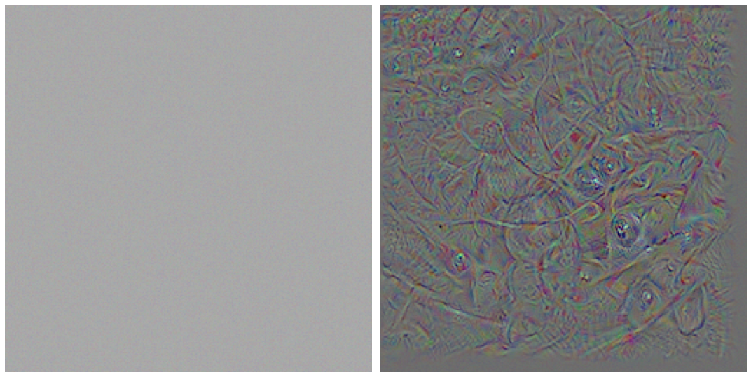
For most ImageNet categories, the preceeding approach does not yield very recognizable images. Features of a given category are often muddled together or dispered throughout the generated input. Below is a typical result, in this case when ‘ant’ is chosen (class_index = 310). The initial random image is transformed as the class activation (logit) increases for the appropriate index. Logits for the model (InceptionV3) given the input to the left are displayed as a scatterplot, with the desired output in red.
A minority of classes do have vaguely recognizable images generated: when we use the category ‘washing machine’ as our target, the glass covers of side-loading washing machines are represented as small round objects in distorted rectangles.
The second Bayesian prior we will enforce is that images will not be too variable from one pixel to the next. Reducing variability between adjacent pixels increases their correlation correlation with each other (see here for an account on pixel correlation here) such that that neighboring pixels are constrained to resemble each other, in effect smoothing out an image. One way to reduce variability between nearby pixels is to perform a convolution, the same operation which our model uses judiciously in neural network form for image classification. For an introduction to convolutions in the context of deep learning, see this page
One choice for convolution is to use a Gaussian kernal with a 3x3 size. The Gaussian distribution has a number of interesting properties, and arguably introduces the least amount of information in its assumption. A Gaussian distribution in two dimensions $x, y$ is as follows:
\[G(x, y) = \frac{1}{2 \pi \sigma^2} \mathrm{exp} \left( \frac{x^2 + y^2}{2 \sigma^2} \right)\]where $\sigma$ is the standard deviation, which we can specify. Using the functional Gaussian blur module of torchvision, the default value for a 3x3 kernal is $\sigma=0.8$ such that the kernal we will use is to a reasonable approximation
where the $1/2$ and $1/4$ values are more precisely just over $201/400$ and $101/400$.
Here we apply a Gaussian convolution to the input in a curriculum in which our convolution is applied at every iteration until three quarters the way through gradient descent, at which time it is no longer applied for the remaining iterations. Heuristically this should a general shape to form before details are filled in.
def generate_input(model, input_tensors, output_tensors, index, count):
	max_iterations = 100
	for i in range(max_iterations):
		...
		if i < (max_iterations - max_iterations/4):
			single_input = torchvision.transforms.functional.gaussian_blur(single_input, 3)
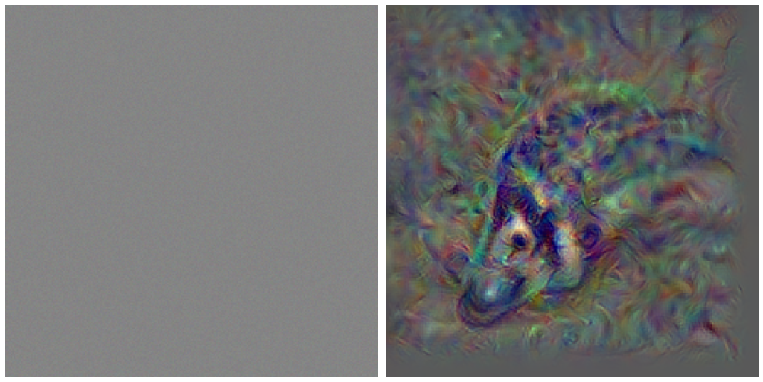
Choosing to optimize for a classification of ‘ant’ (class_index = 310) once again, we see that this smoothness prior leads to a more unstable class prediction but a more realistic generated image of an ant.
Smoothness along leads to a number of more recognizable images being formed,
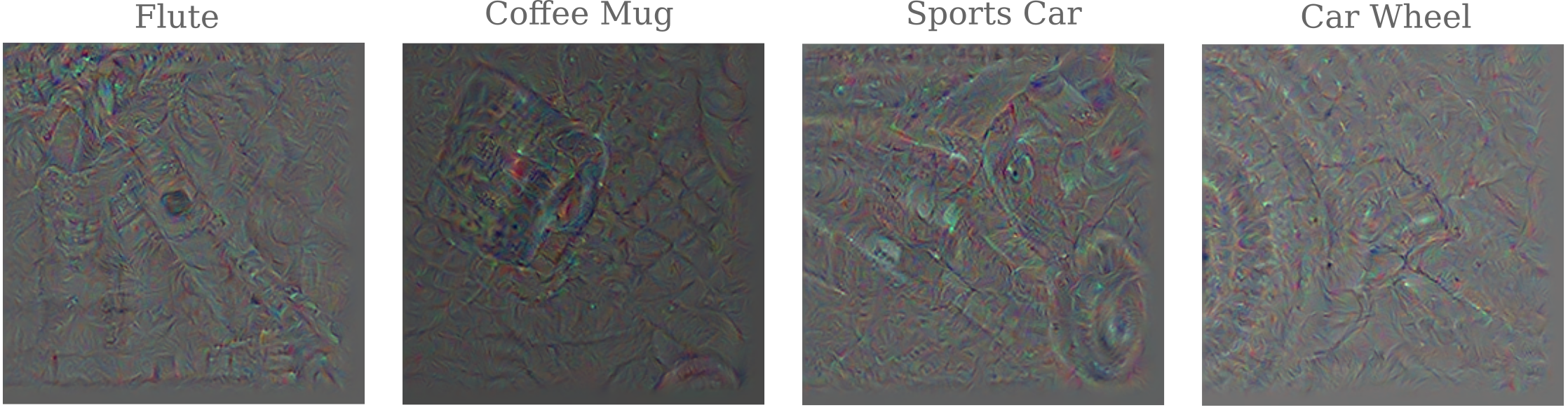
Observe that these images are somewhat dim. This results from the presence of spikes in pixel intensity for very small regions, which the smoothing process does not completely prevent. The rest of the images using the smoothness prior alone (but no others) displayed below have been adjusted for brightness and contrast for clarity.
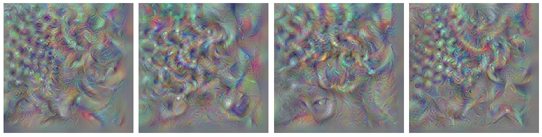
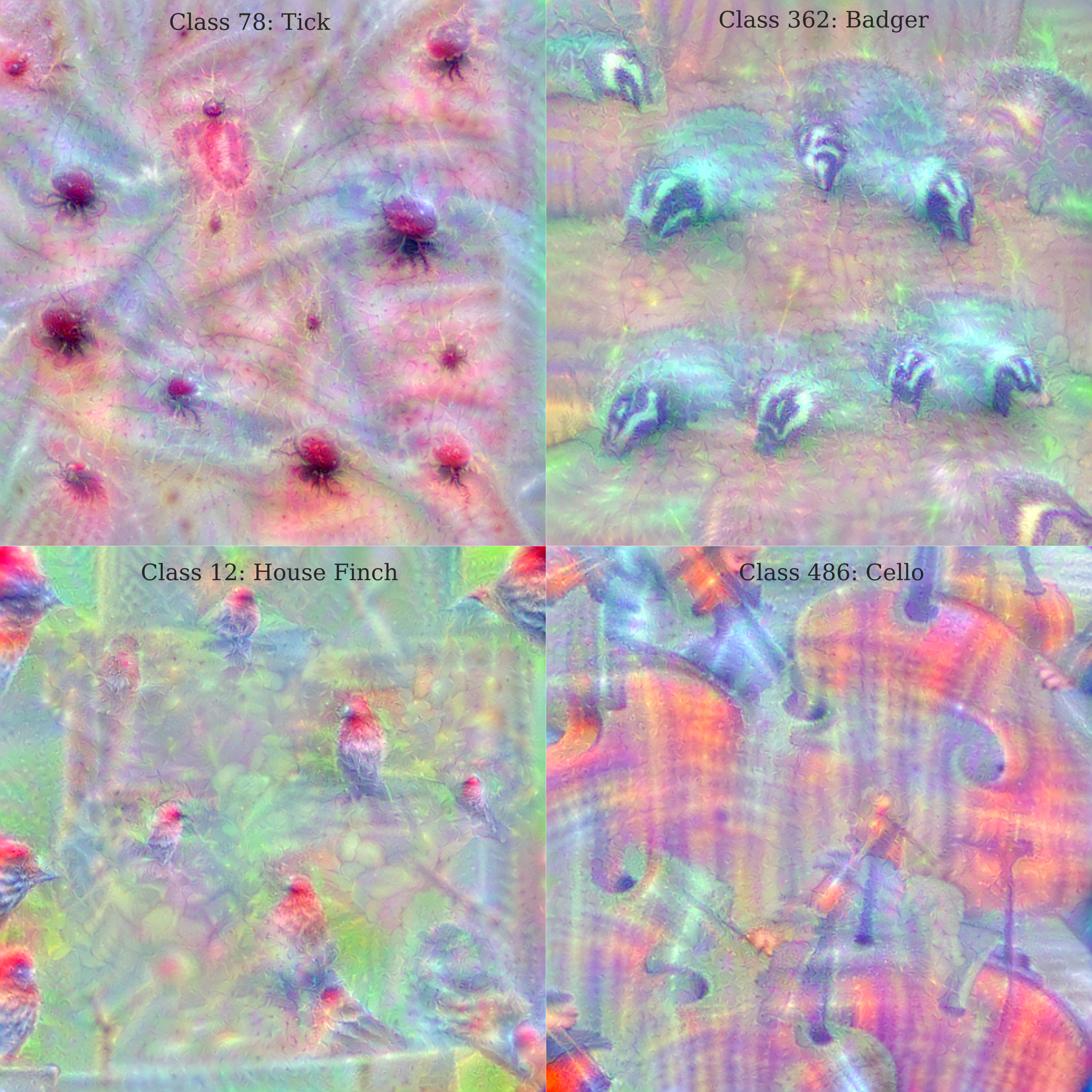
Depending on the initial input given to the model, different outputs will form. For a target class of ‘Tractor’, different initial inputs give images that tend to show different aspect of a tractor: sometimes the distinctive tyre tread, sometimes the side of the wheel, sometimes the smokestack is visible.
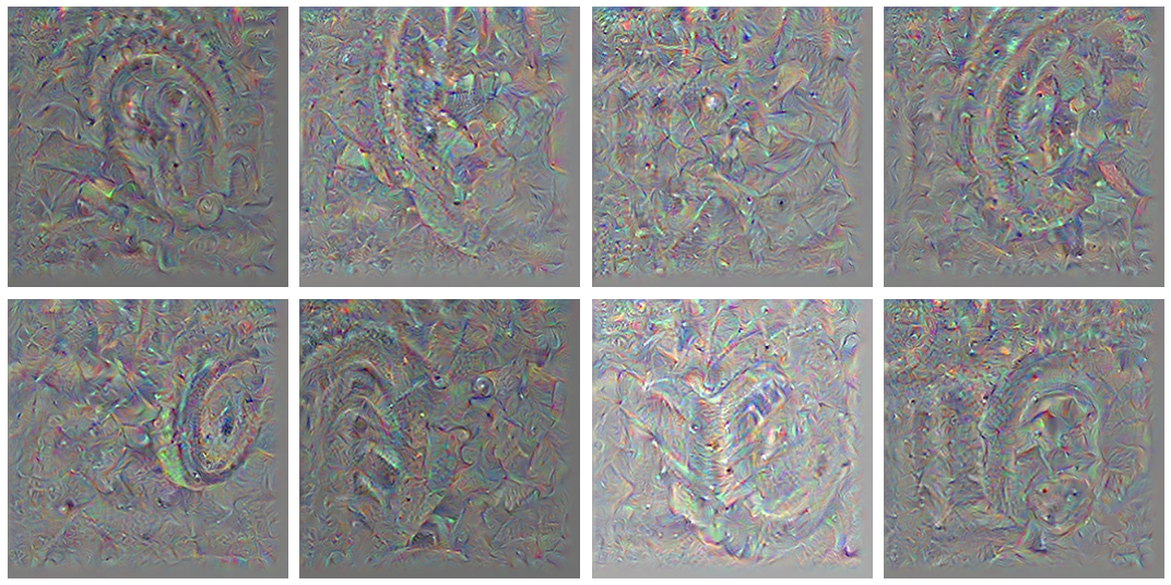
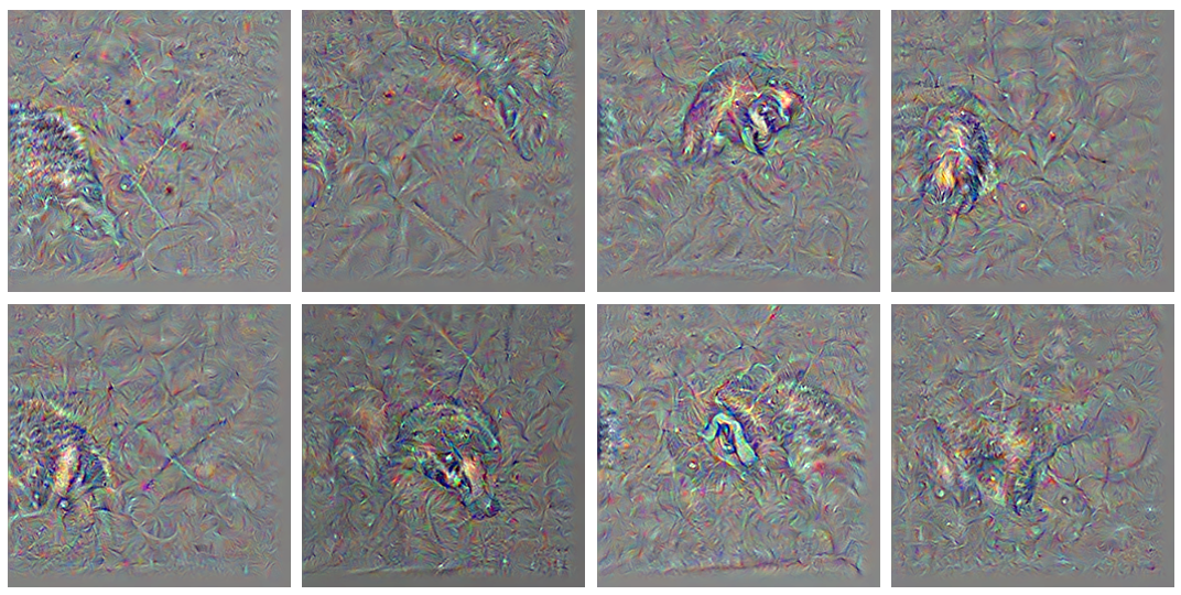
This is perhaps in part the result of the ImageNet training set containing images where not the entire tractor is visible at once. This appears to be a typical result for this image generation technique: if we optimize for ‘Badger’, we usually see the distinctive face pattern but in a variety of orientations
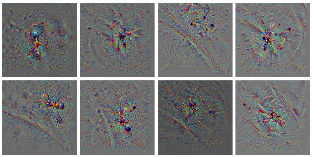
Here for ‘Ant’ we have
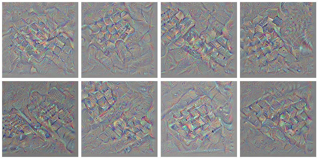
although for other classes, few perspectives are reached: observe that for ‘Keyboard’ the geometry of the keys but not the letters on the keys are consistently generated.
Generating Images using Transformation Resiliency
Next we will add transformational resiliency. The idea here is that we want to generate images that the model does not classify very differently if a small transformation is applied. This transformation could be a slight change in color, a change in image resolution, a translation or rotation, among other possibilities. Along with a Gaussian convolution, we also apply to the first three quarters of all images one of five re-sizing transformations.
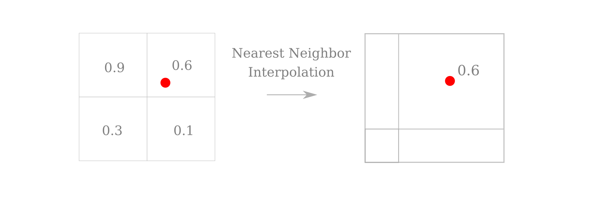
Re-sizing may be accomplished using the torch.nn.functional.interpolate() module, which defaults to a interpolation mode of nearest neighbors. This is identical to the k-nearest neighbors algorithm with a value of $k=1$ fixed. For images, the value of the center of a pixel is taken to be the value across the area of the entire pixel such that the new pixel’s center always lies inside one pixel or another (or on a border). To make this clearaer, suppose we were down-sampling an image by a factor of around 1.5. For the new pixel centered on a red dot for clarity, there is
In addition, a small intensity change is applied to each pixel at random for each iteration using torchvision.transforms.ColorJitter(c) where c is a value of choice. Specifically, $\epsilon \in [-c, c]$ is added to element $a_{x, y}$ of input $a$ to make element $a_{x, y}’= a{x, y} + \epsilon$ of a transformed input $a’$. In the code sample below, we assign $\epsilon \in [0.0001,0.0001]$ but this choice is somewhat arbitrary. Note that this transformation may also be undertaked with much larger values (empirically up to around $\epsilon = 0.05$) and for color, contrast, and saturation as well as brightness by modifying the arguments to torchvision.transforms.ColorJitter().
One note of warning: torchvision.transforms.ColorJitter() is a difficult method for which to set a deterministic seed. random.seen(), torch.set_seed(), and np.seed() together are not sufficient to make the color jitter deterministic, so it is not clear how exact reproduction would occur using this method. If a deterministic reproduction is desired, it may be best to avoid using this module.
def generate_input(model, input_tensors, output_tensors, index, count):
	max_iterations = 100
	for i in range(max_iterations):
		...
		single_input = torchvision.transforms.ColorJitter(0.0001)(single_input)
		if i < 76:
			...
			if i % 5 == 0:
				single_input = torch.nn.functional.interpolate(single_input, 256)
			elif i % 5 == 1:
				single_input = torch.nn.functional.interpolate(single_input, 198)
			elif i % 5 == 2:
				single_input = torch.nn.functional.interpolate(single_input, 160)
			elif i % 5 == 3:
				single_input = torch.nn.functional.interpolate(single_input, 180)
			elif i % 5 == 4:
				single_input = torch.nn.functional.interpolate(single_input, 200)
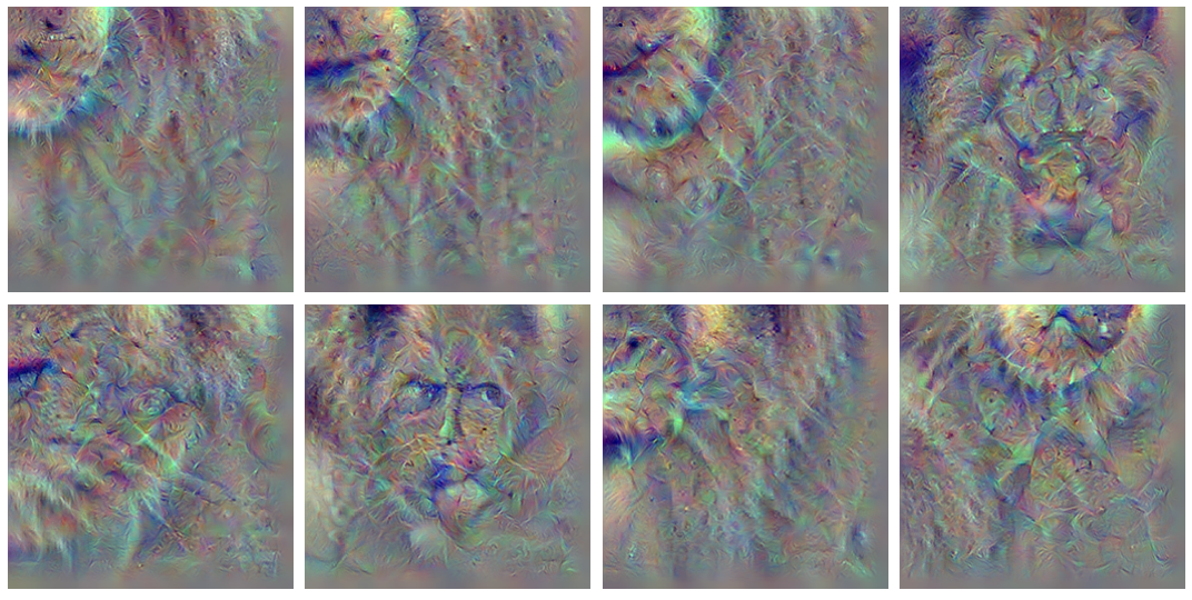
The class label (and input gradient) tends to be fairly unstable during training, but the resulting images can be fairly recognizable: observe the lion’s chin and mane appear in the upper left hand corner during input modification.
Note that much of the fluctuation in the class activation scatterplot to the right is due to the change in input image resolution, which changes the activation value for each class even if it does not change the relative activation values of the target class compared with the others.
There is a noticeable translation in the image from the top left to the bottom right during the initial 75 iterations with the function above. This is the result of using nearest neighbor interpolation while resampling using torch.nn.functional.interpolate. It appears that in the case where multiple pixels are equidistant from the target, the upper left-most pixel is chosen as the nearest neighbor. When downsampling an input, we are guaranteed to have four pixels that are nearest neighbors to the new pixels.
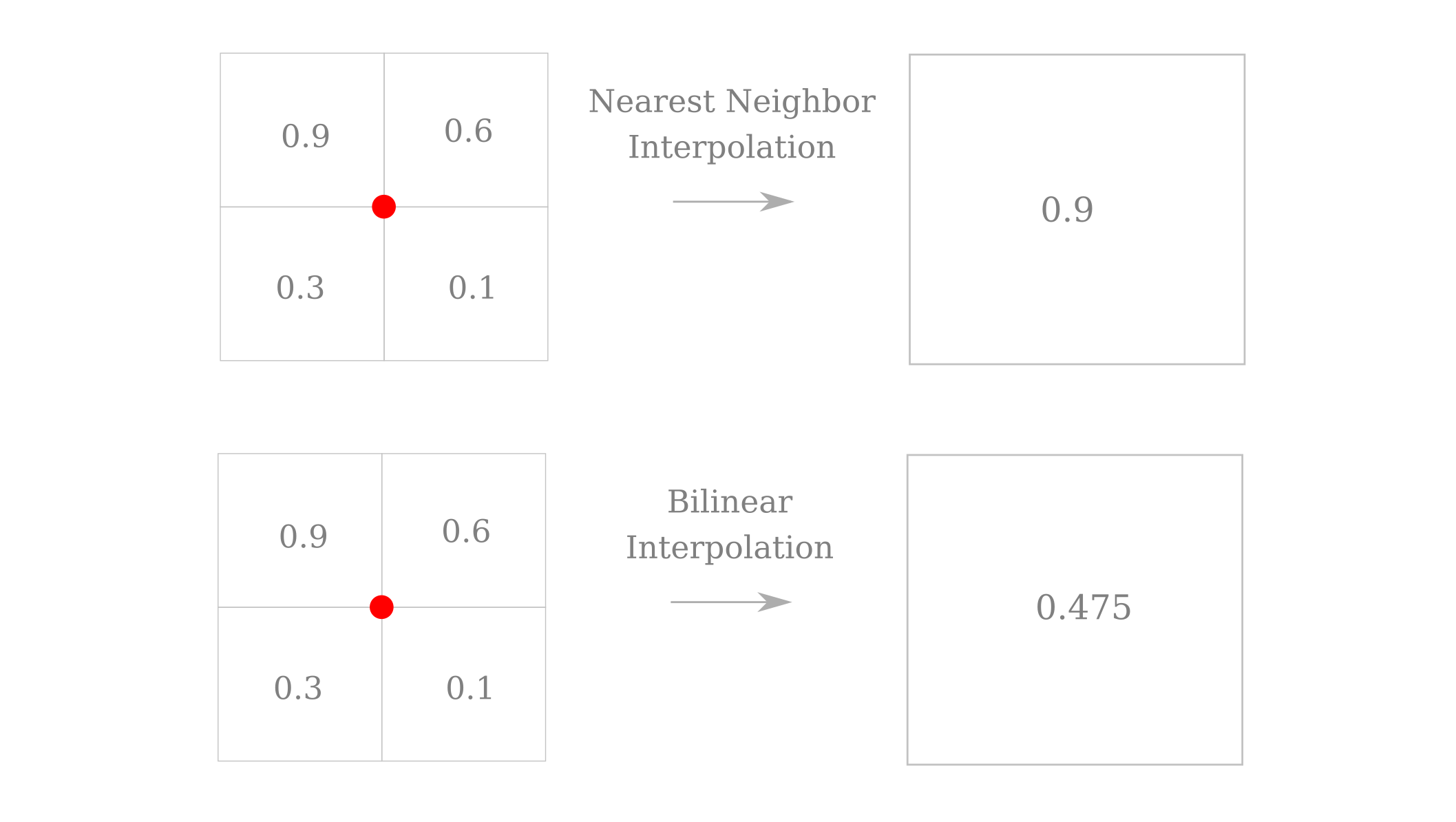
This can be remedied by choosing an interpolation method that averages over pixels rather than picking only one pixel value. The following diagram illustrates the upper-left nearest neighbor interpolation method compared to a bilinear interpolation. Note how the upper left pixel becomes centered down and to the right of its original center for nearest neighbor interpolation, whereas in contrast the bilinear interpolation simply averages all pixels together and does not ‘move’ the top left value to the center.
We therefore have a method that effectively translates as well as resizes our original images, which is applied in addition to the Gaussian convolution and jitter mentioned above. For around half of our 16 random input we get a recognizable lion face and mane, and for others a paw is found
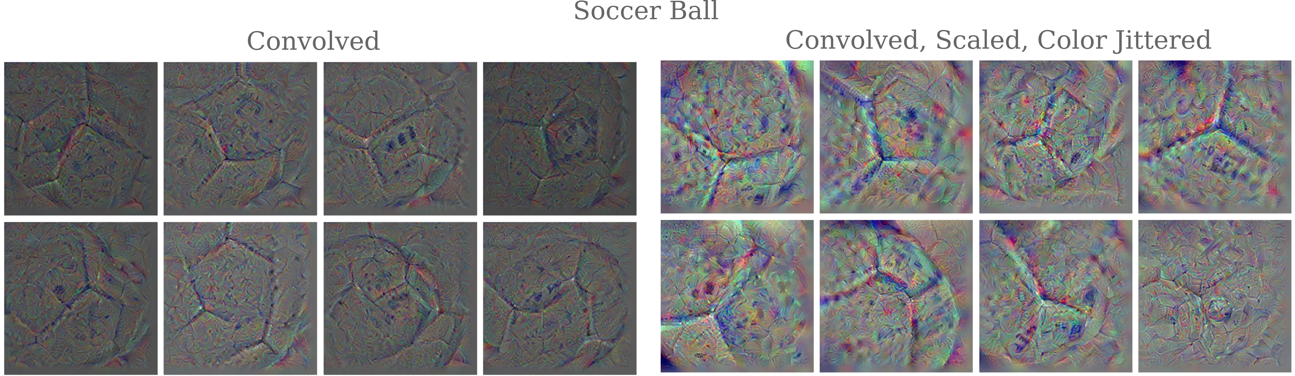
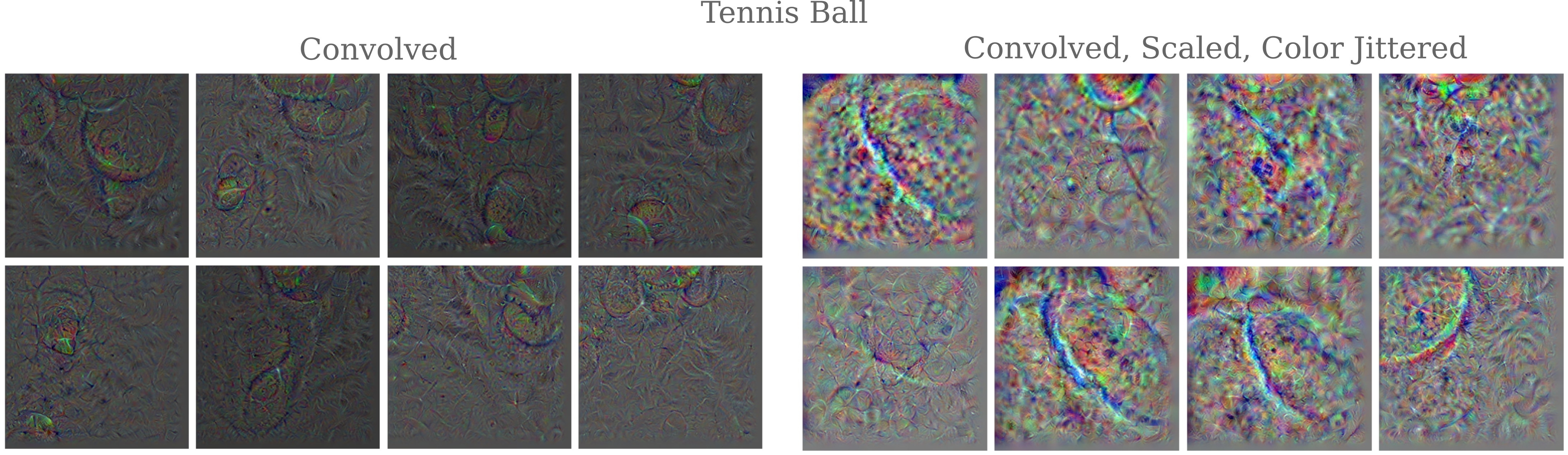
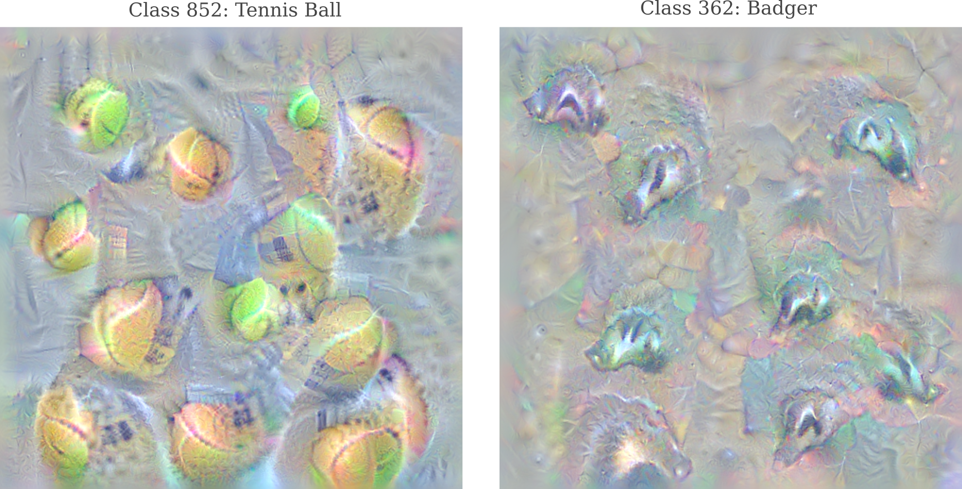
We can compare the effects of adding transformations to the modification process to the resulting image. Here the convolved (such that smoothness is enforced) images are not adjusted for brightness and contrast as they were above. The figures below demonstrates ho how re-sizing during input modification effectively prevents spikes in pixel intensity. For a soccer ball and a tennis ball, we have
Some inputs are now unmistakeable, such as this badger’s profile
or ‘Chainmail’
Note, however, that transformational invariance does not necessarily lead to a noticeable increase in recognizability for all class types.
Image Transfiguration
It is worth appreciating exactly what we were able to do in the last section. Using a deep learning model trained for image classification combined with a few general principles of how natural images should look, we were able to reconstruct a variety of recognizable images representing various desired classes.
This is remarkable because the model in question (InceptionV3) was not designed or trained to generate anything at all, merely to make accurate classifications. Moreover, the initial input being used as a baseline for image generation (a scaled uniform or normal random distribution) is quite different from anything that exists in the training dataset Imagenet, as these are all real images. What happens if we start with a real image and then apply our input gradient descent method to that? This process will be termed ‘transfiguration’ on this page to avoid confusion with ‘transformation’, which is reserved for the jitters, interpolations, rotations, and translations applied to an input.
To begin with, it may be illuminating to perform a control experiment in which the input is the same as the targeted class. In this case we would expect to simply see an exaggeration of the features that distinguish the object of the class compared to other classes. Applying our transformation-resistatant and Gaussian-convolved input gradient method to images of dalmations that are not found in the original Imagenet training dataset, we have
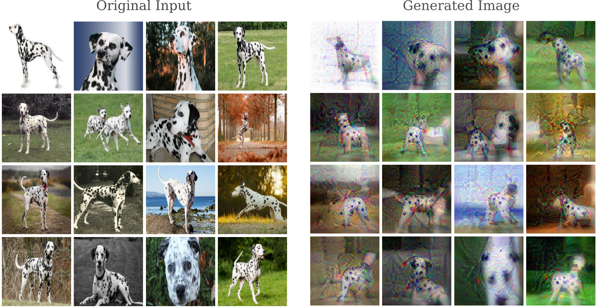
The dalmatian’s spots are slightly exaggerated, but aside from some general lack of resolution the dalmatians are still clearly visible. Now let’s make a relatively small transfiguration from one breed of dog to another. Beginning again with images of dalmatians but this time performing the input gradient procedure with a target class of ‘Siberian Husky’ we have
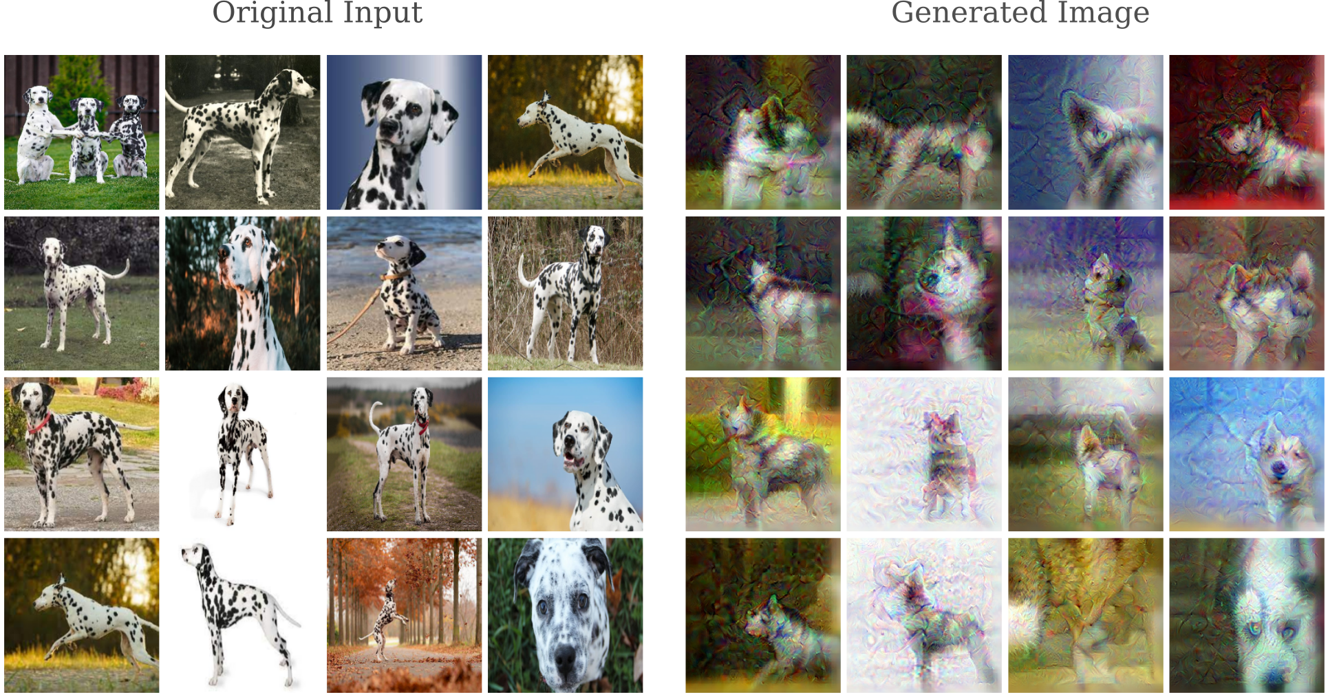
The spots have all but disappeared, replaced by thicker fur and the grey stripes typical of Huskies. Note how even smaller detailes are changed: in the bottom right, note how the iris color changes from dark brown to light blue, another common Husky characteristic.
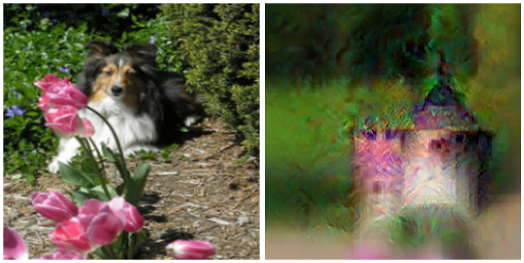
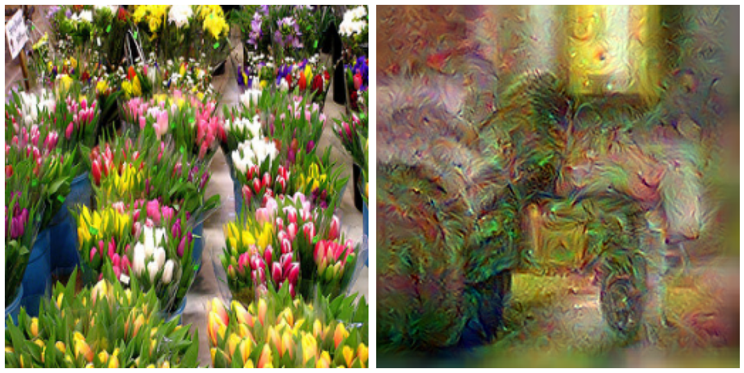
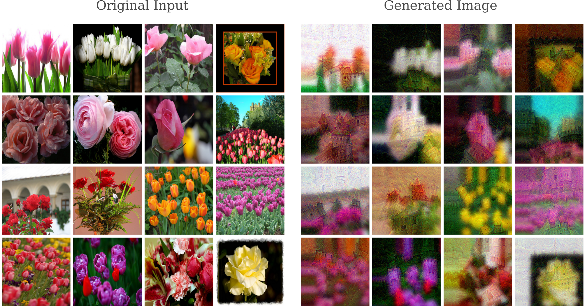
Transforming an input from one breed of dog to another may not seem difficult, but the input gradient procedure is capable of some very impressive changes. Here we begin with images of flowers and target the ‘Castle’ class
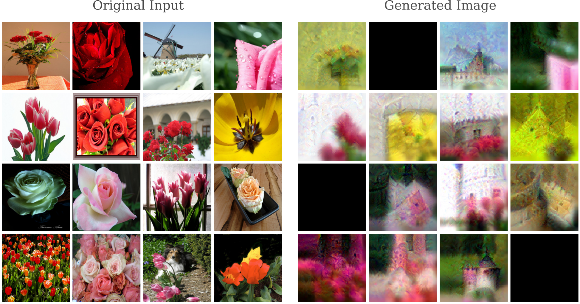
We can get an idea of how this process works by observing the changes made to the original image as gradient descent occurs. Here over the 100 iterations of transfiguration from a flower (‘flowerpot’ class in green on the scatterplot in the right) to a ‘Castle’ target class (the red dot on the right)
Even with as substantial a change as a flower to a castle some outputs are unmistakable, such as this castle tower.
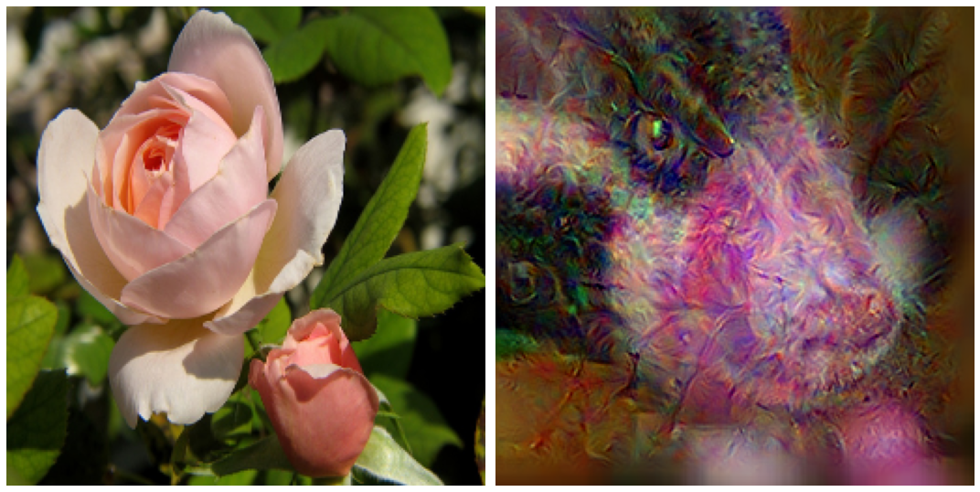
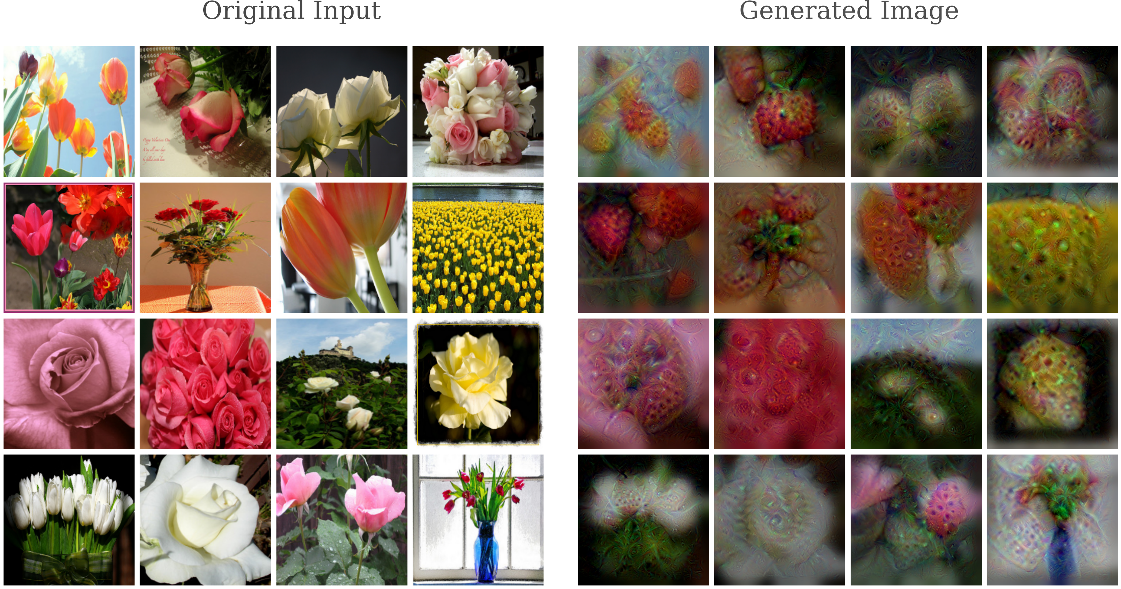
Other transfigurations are possible, such as this badger from a rose bush
or this tulip bed into a ‘Tractor’
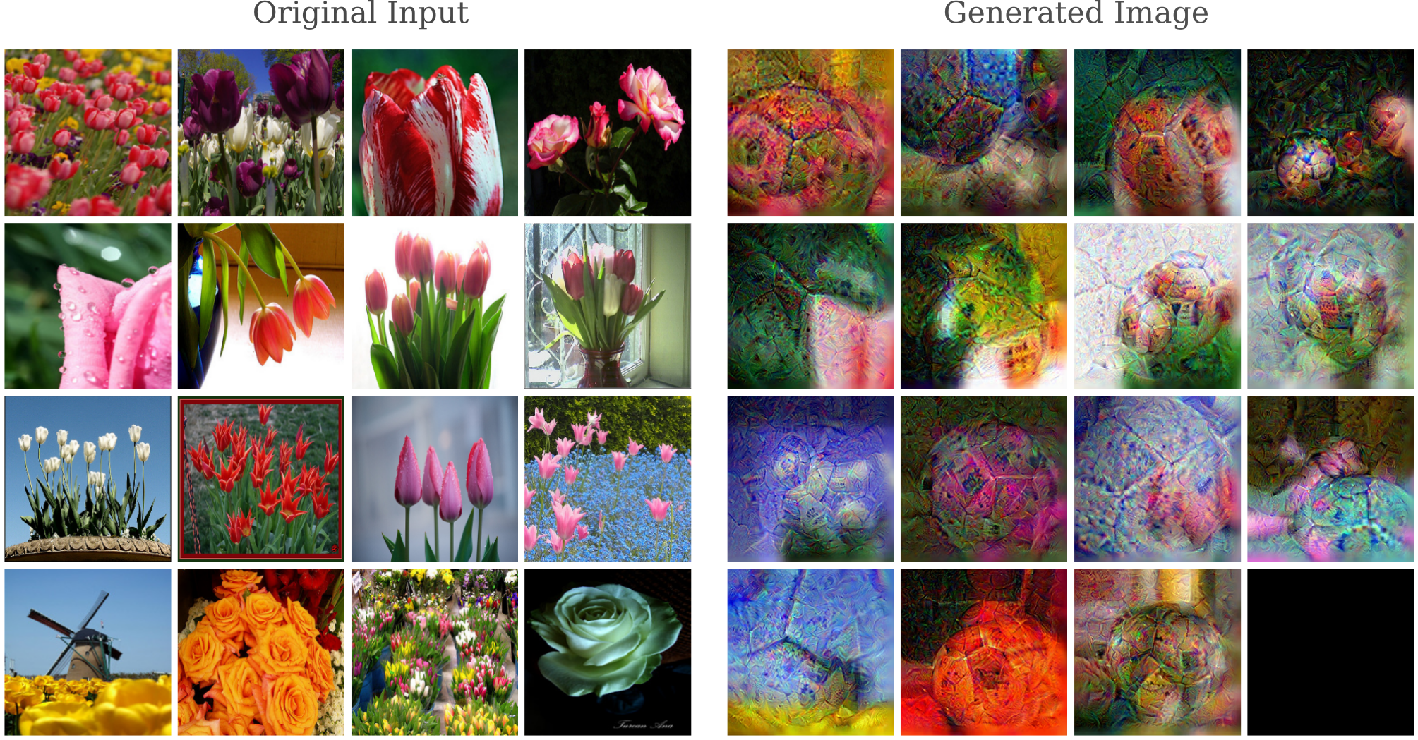
or these flowers transfigured into ‘Soccer ball’.
Earlier it was noted that image resizing with torch.nn.functional.interpolate() leads to translation when downsampling the input. This can be avoided by switching the interpolation mode away from nearest neighbor, to instead average either using a bilinear or bicubic method. This can be done in torch.nn.functional.interpolate() by specifying the correct keyword argument, or else we can make use of the module torchvision.transforms.Resize(), which defaults to bilinear mode. The latter is the same method we used to import our images, and was employed below. Notice how there is now no more translation in the input image.
Input Generation with Auxiliary Outputs
We have seen how representatives of each image class of the training dataset may be generated using gradient descent on the input with the addition of a few reasonable priors, and how this procedure is also capable of transforming images of one class to another. Generation of an image matching a specific class requires an output layer trained to perform this task, and for most models this means that we are limited to one possible layer. But InceptionV3 is a somewhat unique architecture in that it has another output layer, called the auxiliary output, which is employed during training to stabilize gradients and then deactivated during evaluation with model.eval() if one is using Pytorch.
Let’s investigate whether we can perform gradient descent to generate images using this auxiliary output rather than the usual output layer. The architecture we want to use is
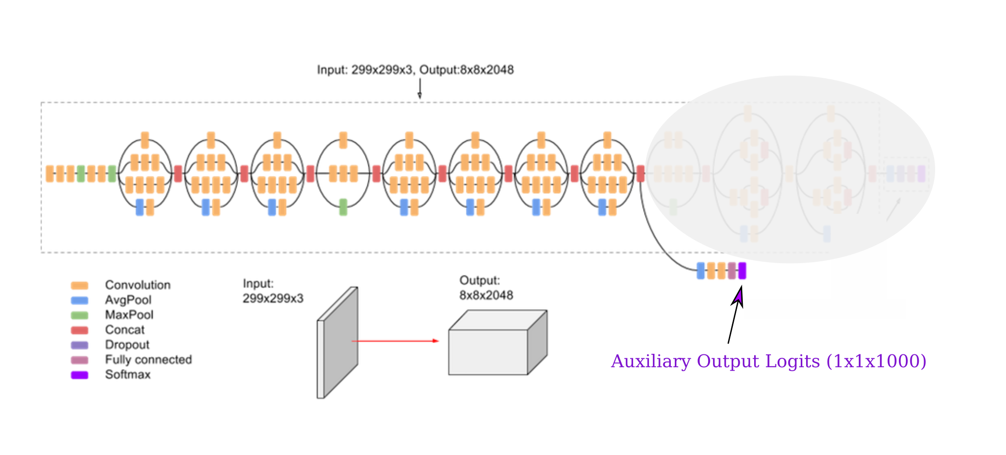
Note that the Pytorch implementation of the above architecture does not include the softmax layer on either the auxiliary or main output.
It may be worth exploring some history behind how different deep learning libraries perform differentiation. The original Torch library employed symbol-to-number differentiation, which was also employed by Caffe. In this approach, the derivatives (in the form of Jacobian matricies) of each layer are specified at the start of runtime, and computed to form numerical values for each node upon forward and backpropegation. This approach is in contrast to symbolic differentiation, in which extra nodes are added to each model node (ie layer) that provides a symbolic description of the derivatives of those nodes. The computational graph for performing backpropegation is identical between these two approaches, but the former hides the graph itself and the latter exposes it at the expense of extra memory. The latter approach was taken by libraries like Theano and Tensorflow.
To this author’s knowledge, however, these differences have blurred with the more modern incarnations of Tensorflow and Pytorch. Pytorch now uses a method called automatic differentiation, which attempts to combine the speed of numerical differentiation with the stability and flexibility of symbolic differentiation.
We wish to back-propegate from a leaf node of our model, but this node is not returned as an output during evaluation mode. Switching to training mode is not an option because the batch normalization layers of the model will attain new parameters, interfering with the model’s ability to classify images.
In symbolic differentiation -based libraries, computing the gradient of the input with respect to a layer that is not the output is relatively straightforward: the output and loss from the specific layer of interest are specified, and backpropegation can then proceed directly from that layer. But in Pytorch this is not possible, as all we would have from an internal node is a number representing the gradient with respect to the output, rather than instruction for obtaining a gradient from that node itself.
So instead we must modify the model itself. If we were not using an open-source model this would not be feasible, but as we are indeed using a freely accessible model we can do this a number of different ways. One way is to make a new class that inherits from nn.Module and is passed as an initialization argument the original Inceptionv3 model. We then provide a new forward() method that modifies the original inceptionv3 method (located here) such that the layer of choice is returned.
class NewModel(nn.Module):

	def __init__(self, model):
		super().__init__()
		self.model = model

	def forward(self, x):
		# N x 3 x 299 x 299
		x = self.model.Conv2d_1a_3x3(x)
		# N x 32 x 149 x 149
		x = self.model.Conv2d_2a_3x3(x)
		# N x 32 x 147 x 147
		x = self.model.Conv2d_2b_3x3(x)
		# N x 64 x 147 x 147
		x = self.model.maxpool1(x)
		# N x 64 x 73 x 73
		x = self.model.Conv2d_3b_1x1(x)
		# N x 80 x 73 x 73
		x = self.model.Conv2d_4a_3x3(x)
		# N x 192 x 71 x 71
		x = self.model.maxpool2(x)
		# N x 192 x 35 x 35
		x = self.model.Mixed_5b(x)
		# N x 256 x 35 x 35
		x = self.model.Mixed_5c(x)
		# N x 288 x 35 x 35
		x = self.model.Mixed_5d(x)
		# N x 288 x 35 x 35
		x = self.model.Mixed_6a(x)
		# N x 768 x 17 x 17
		x = self.model.Mixed_6b(x)
		# N x 768 x 17 x 17
		x = self.model.Mixed_6c(x)
		# N x 768 x 17 x 17
		x = self.model.Mixed_6d(x)
		# N x 768 x 17 x 17
		x = self.model.Mixed_6e(x)
		# N x 768 x 17 x 17
		aux = self.model.AuxLogits(x)
		return aux
One important thing to note is that the Inceptionv3 module is quite flexible with regards to the input image size when used normally in evaluation mode, but now that we have modified the network it must be given images of size 299x299 or the dimensions of the hidden layers will not align with what is required. This can be enforced by something as straightforward as
image = torchvision.transforms.Resize(size=[299, 299])(image)
in the __getitem__() special method of our data loader (see the source code for more information).
The gradients in this layer also tend to be slightly smaller than the original output gradients, so some re-scaling of our gradient descent constant $\epsilon$ is necessary. For clarity, at each iteration of our descent starting with input $a_n$, we make input $a_{n+1}$ by finding the L1-normalized loss of the auxiliary output layer $O’(a; \theta)$ with respect to the desired output $\widehat{y}$,
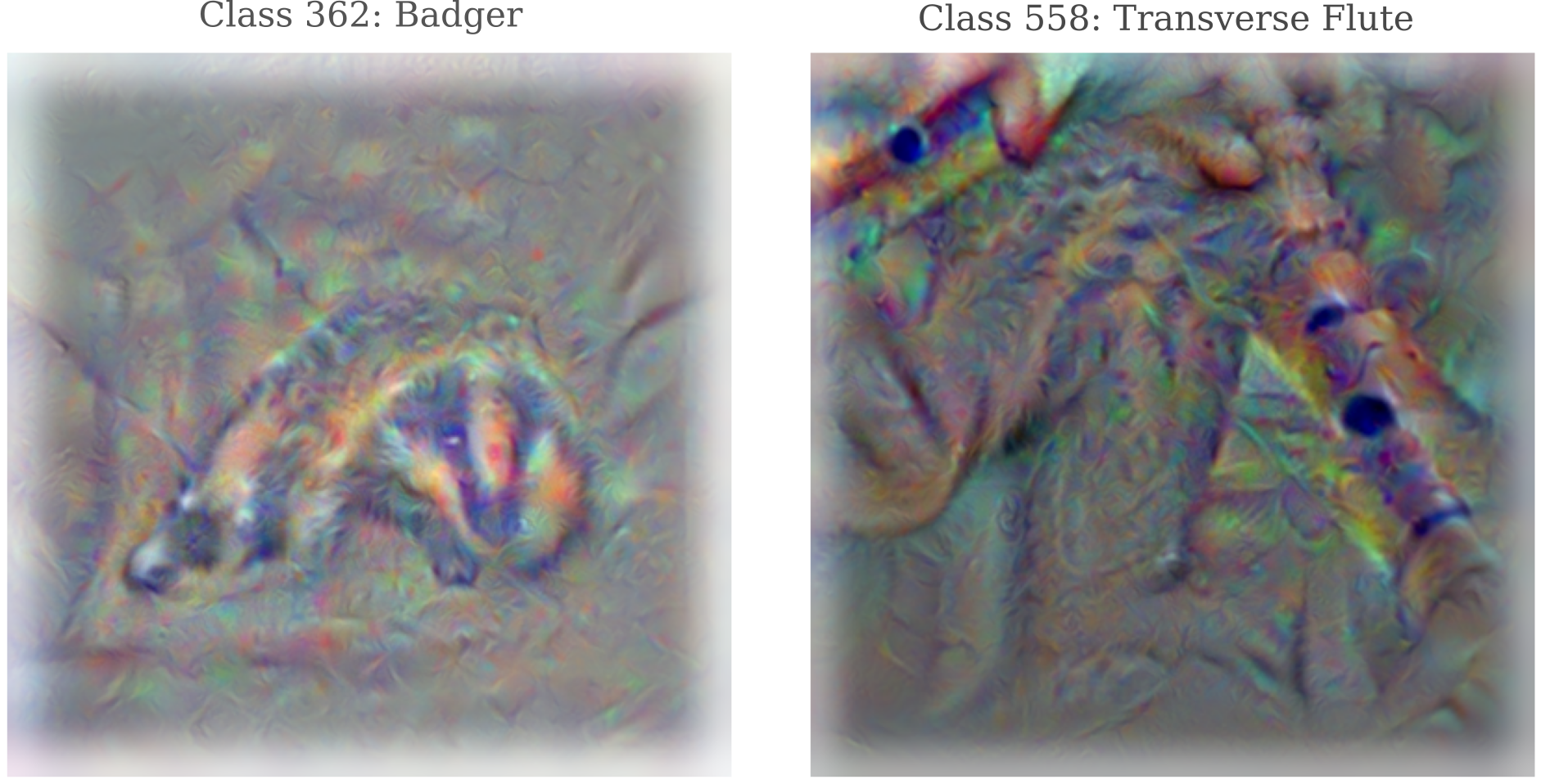
\[a_{n+1} = a_n - \epsilon \nabla_a J(O'(a; \theta), \widehat{y})\]The results are interesting: perhaps slightly clearer (ie higher resolution) than when we used the normal output layer, but maybe less organized as well.
Jitter using Cropped Octaves
The generated images shown so far on this page exhibit to some extent or another the presence of high-frequency patterns, which can be deleterious to the ability to make an image that is accurate to a real-world example. High frequency between image pixels often appears as areas of bright dots set near each other, or else sometimes as dark lines that seem to overlay light regions. The wavy, almost ripple-like appearance of some of the images above appears to be the result of application of smoothing (via Gaussian kernal convolution or re-sizing) to the often chaotic and high-frequency gradient applied to the images during generation.
One way to address the problem of high frequency and apparent chaos in the input gradient during image generation is to apply the gradient at different scales. This idea was pioneered in the context of feature visualization by Mordvintsev and colleages and published in the Deep dream tutorial, and is conceptually fairly straightforward: one can observe that generated images (of both features or target classes) have small-scale patterns and large-scale patterns, and often these scales do not properly interact. When a lack of interaction occurs, the result is smaller versions of something that is found elsewhere in the images, but in a place that reduces image clarity. The idea is to apply the gradient to different scales of the input image to address this issue.
One octave interval is very much like the gradient descent with Gaussian convolution detalied earlier. The main idea compared to the previous technique of image resizing is that the image is up-sampled rather than down-sampled for higher resolution, and that this up-sampling occurs in discrete intervals rather than at each iteration. Another difference is that instead of maintaining a constant learning rate $\epsilon$ and Gaussian convolution standard deviation before removing the convolution, both are gradually decreased as iterations increase.
There are a number of different ways that octave-based gradient descent may be applied, but here we choose to have the option to perform gradient descent on a cropped copy of the input image, and apply a Gaussian convolution to the entire image at each step (rather than only to the portion that was cropped and modified via gradient descent). This approach is similarto a positional jitter method that has been used elsewhere, but incorperates an increase in scale at specific stages of the positional jitter.
def octave(single_input, target_output, iterations, learning_rates, sigmas, size, crop=True):
	...
	start_lr, end_lr = learning_rates
	start_sigma, end_sigma = sigmas

	for i in range(iterations):
		if crop:
			cropped_input, crop_height, crop_width = random_crop(single_input.detach(), size)
		else:
			cropped_input, crop_height, crop_width = random_crop(single_input.detach(), len(single_input[0][0]))
			size = len(single_input[0][0])
		single_input = single_input.detach() # remove the gradient for the input (if present)
		input_grad = layer_gradient(Inception, cropped_input, target_output) # compute input gradient
		single_input -= (start_lr*(iterations-i)/iterations + end_lr*i/iterations)*input_grad # gradient descent step
		single_input = torchvision.transforms.functional.gaussian_blur(single_input, 3, sigma=(start_sigma*(iterations-i)/iterations + end_sigma*i/iterations))

	return single_input
Usually multiple octaves are performed during gradient descent, and this can be achieved by chaining the previous function to resized inputs. Here we have three octaves in total, bringing an initial image of size 299x299 to an output of size 390x390.
# 1x3x299x299 input
single_input = octave(single_input, target_output, 100, [1.5, 1], [2.4, 0.8], 0, crop=False)

single_input = torchvision.transforms.Resize([340, 340])(single_input)
single_input = octave(single_input, target_output, 100, [1.3, 0.45], [1.5, 0.4], 320, crop=True)

single_input = torchvision.transforms.Resize([390, 390])(single_input)
single_input = octave(single_input, target_output, 100, [1.3, 0.45], [1.5, 0.4], 390, crop=False)
The results show some increased clarity, but also that images remain somewhat noisy with respect to the colors and textures that are formed.
Note the light grey border on both images above. This is the result of performing Gaussian blurring on the entire image whilst only performing a gradient-based update on a cropped portion, meaning that the areas not included in the crop are blurred but not updated and tend to wash out. These borders may be cropped from the final image or else we may only blur the areas that were updated as follows:
single_input[:, :, crop_height:crop_height+size, crop_width:crop_width+size] -= (start_lr*(iterations-i)/iterations + end_lr*i/iterations)*input_grad
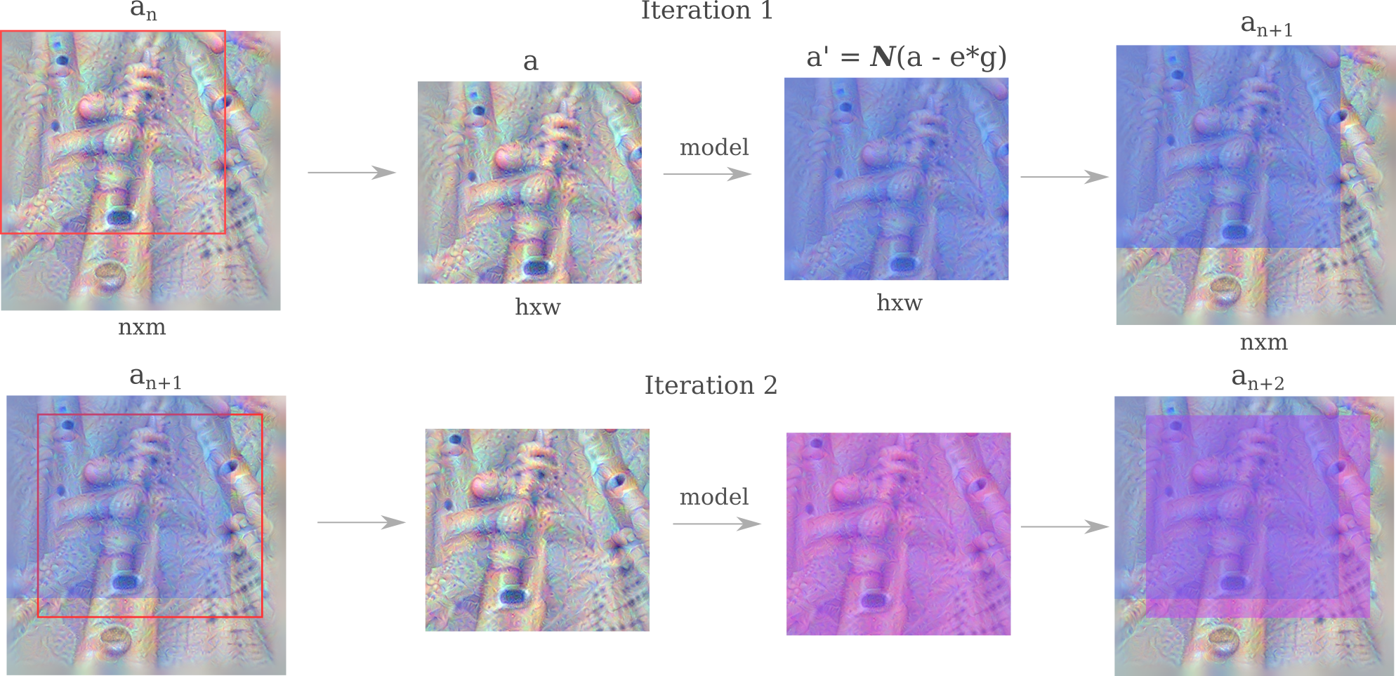
To see how using cropped portions of octaves implements a positional jitter, consider two consecutive updates to an image $a$. The model (InceptionV3 in this case) receives inputs that are small translations of each other (along with the addition of a gradient descent step) such that the gradient $g$ of each input with respect to the output class that is being optimized does not depend on the exact position of each pixel value, only the relative (and approximate) position.
Note that the size of the cropped portion of $a$ that is fed to the model has undetermined dimensions $h$ and $w$. Some model architectures require an input of a fixed size, while others are more flexible. Implementations of models used for experimentation on this page are generally flexible, mostly due to their convolutional and pooling layers. Increasing the $h$ and $w$ resolution of the portion of the image that is used as an input to the model allows for the application of gradients at smaller scales, leading to a more detailed image at the expense of some coherence between portions of the imag
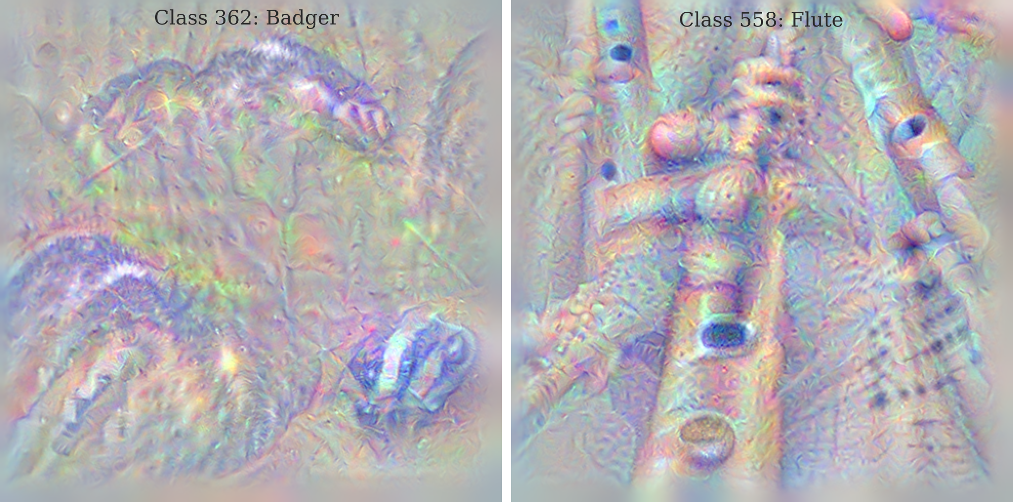
Further optimizing for a coherent input with two cropped octave-based jitters over 720 iterations,
single_input = octave(single_input, target_output, 220, [6, 5], [2.4, 0.8], 0, pad=False, crop=False)

single_input = torchvision.transforms.Resize([490, 490])(single_input)
single_input = octave(single_input, target_output, 500, [1.3, 0.45], [1.5, 0.4], 470, pad=False, crop=True)
gives
GoogleNet Image Generation
In images of inputs generated using gradient descent published by Mordvintsev and colleagues, generated images are generally better-formed and much less noisy than they appear on this page. Øygard investigated possible methods by which these images were obtained (as the previous group did not publish their image generation code) and found a way to produce more or less equivalent images and authored a helpful Github repo with the programs responsible.
Both referenced studies have observed images that are in general clearer than most of the images on this page. Øygard adapted a method modified from an approach in the Tensorflow deep dream tutorial octave method, which resulted in impressively clear images.
A wide array of possible modifications to the octave gradient descent method were attempted with little improvement on the clarity displayed in the last section. This led to the idea that perhaps it is the model itself rather than the optimization method that was responsible for the increased noise relative to what other researchers have found.
The cited works in this section all used the original GoogleNet architecture to generate images. whereas this page has so far focused on the related InceptionV3 model. GoogleNet may be depicted as follows:
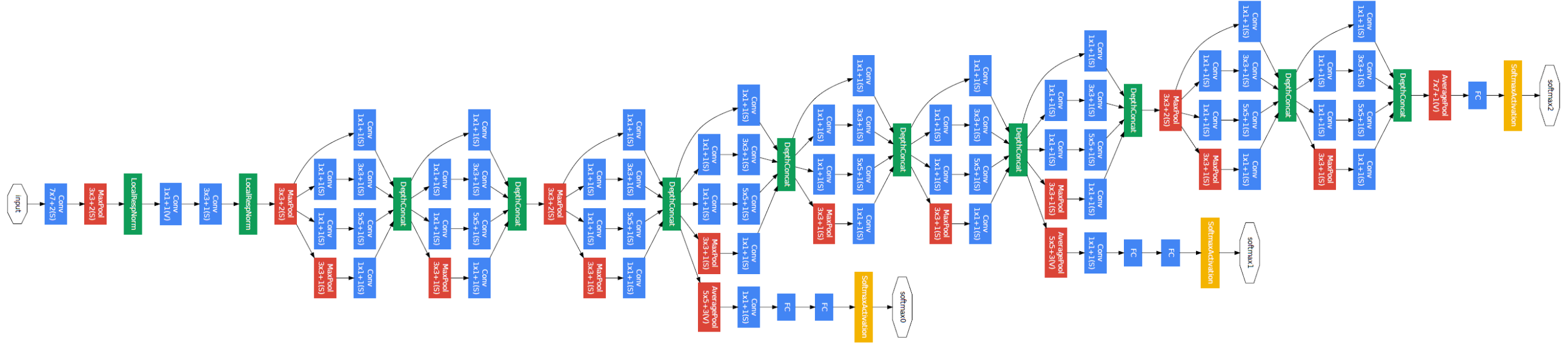
It may be appreciated that this network is a good deal shallower than InceptionV3 (22 versus 48 layers, respectively) but otherwise contains a number of the same general features. One notable change from the original is that the Pytorch version of GoogleNet uses Batch normalization, whereas the original did not.
Optimizing for the ‘Stop Light’ ImageNet class, we now have a much more coherent image in terms of color and patterns over two octaves.
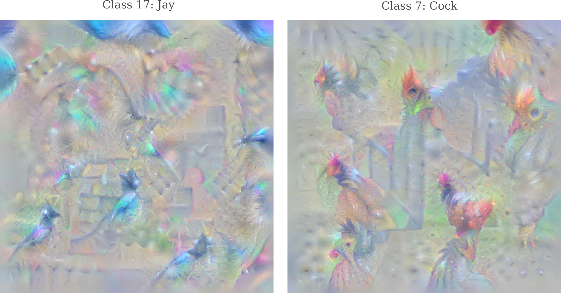
Observing more of the images, we find that our octave-based input generation technique is effective for birds
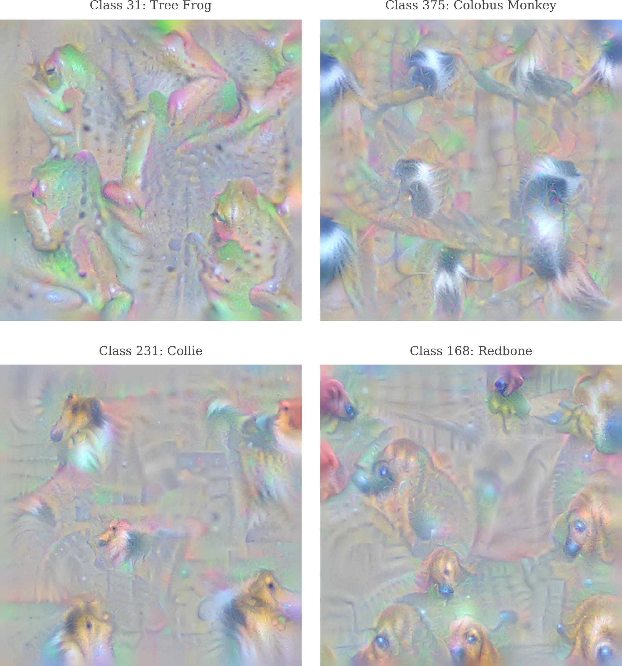
as well as dogs and other animals.
Flames and fires are particularly accurate as well.
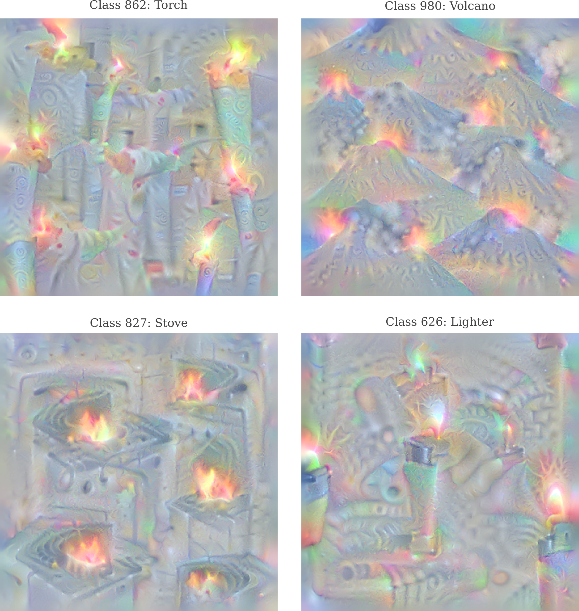
Note how the image generated for ‘stove’ has much larger flames than are realistic. This kind of exaggeration is seen for a number of objects in which there is some differentiating features. On the other hand, the Imagenet dataset has no classes that differentiate faces, and observe how the faces for ‘neck brace’ below are animal-like, not a surprise being that Googlenet will have seen far more dog and other animal faces than human ones.
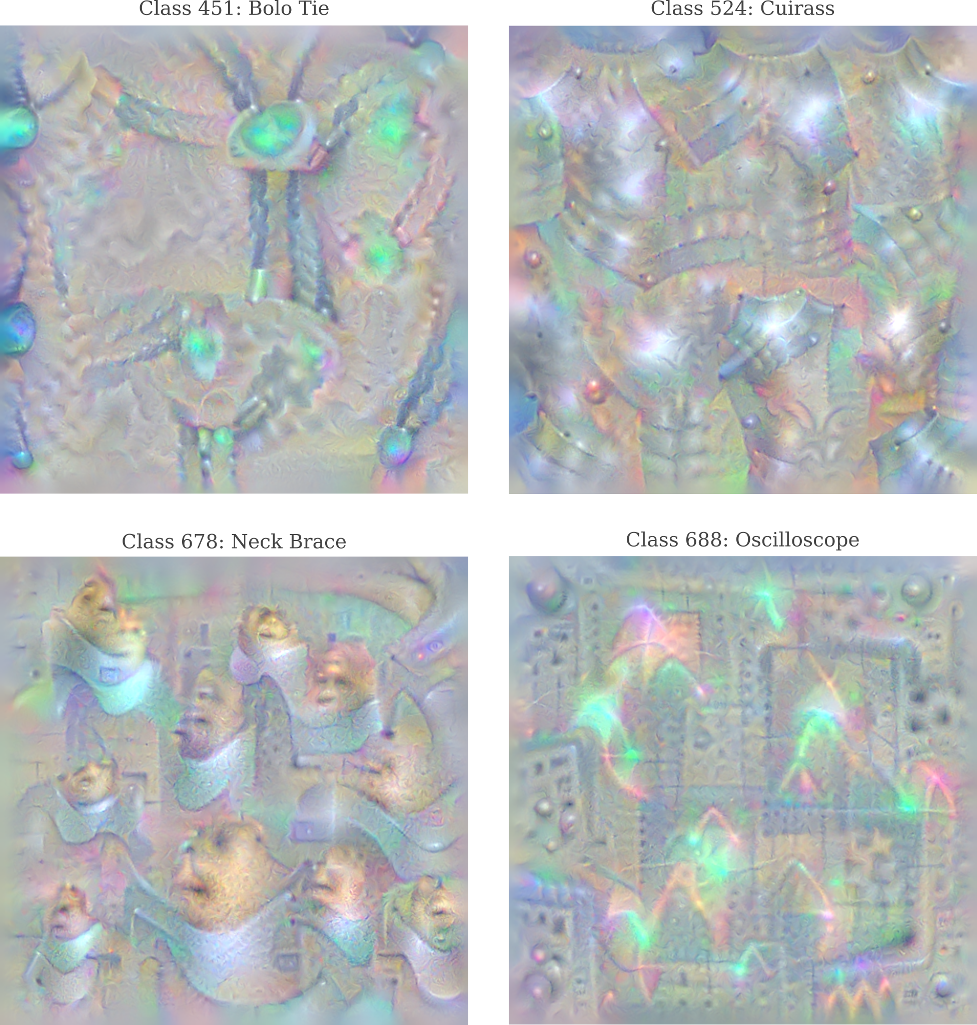
Also observe the fine point accuracy in some of the these images: we even find a sine wave forming in the image of ‘oscilloscope’, and the ‘bolo tie’ even has a silver fastener at the end of the tie.
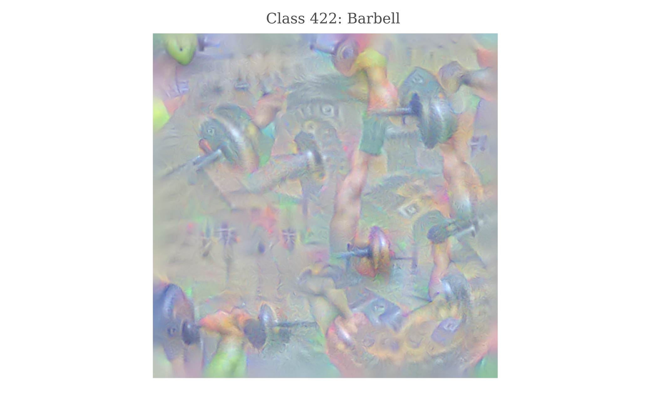
As reported previously, some many of an object contain peripheral features: observe how optimizing for a ‘barbell’ output includes an arm to pick up the barbell.
For generated images of the entire suite of ImageNet classes, see here.
Padding in the first octave
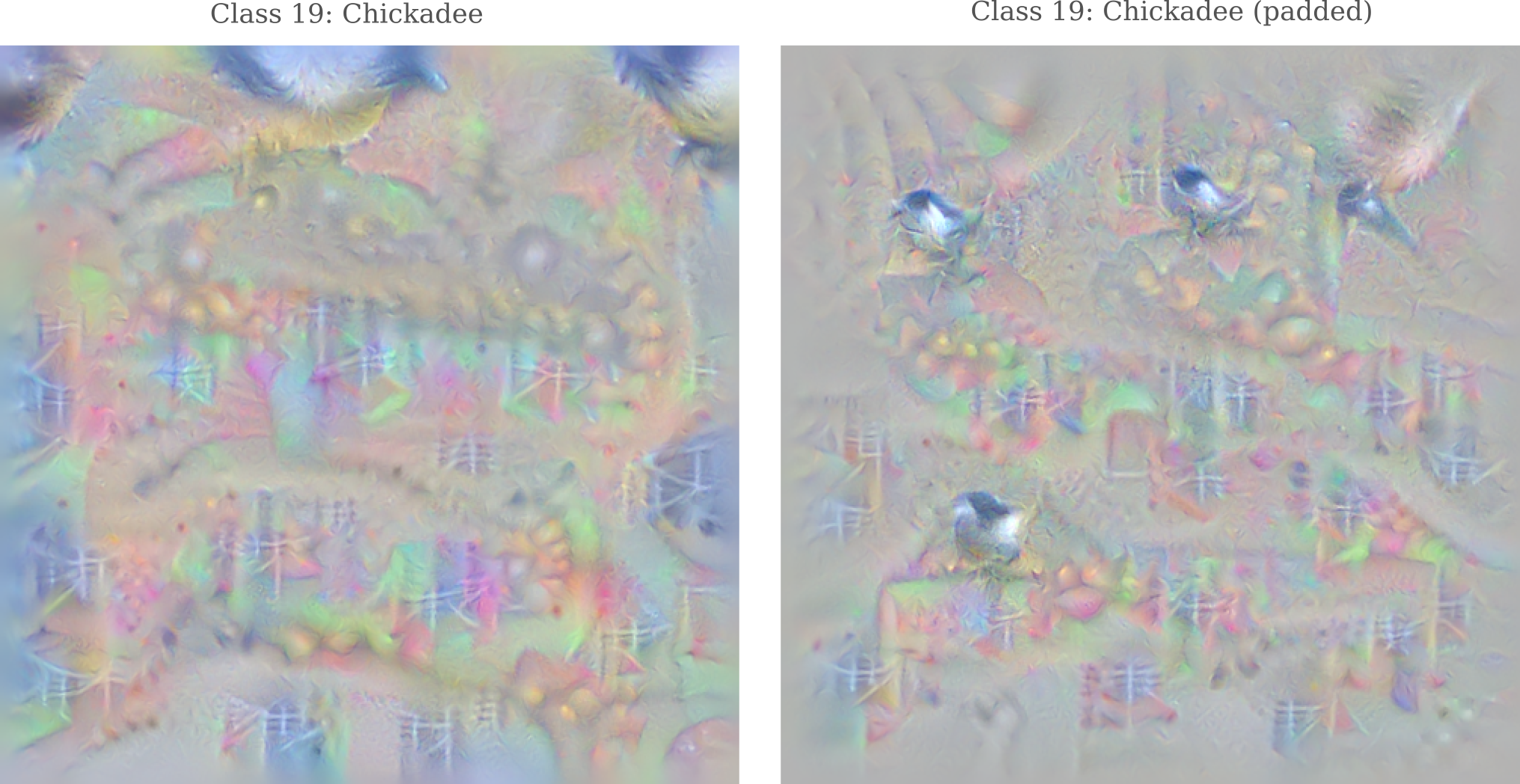
For certain ImageNet classes, generated images tend to have most of their relevant features focused on the periphery, as that is where the gradient is largest. For example, optimizing for class 19 (chickadee) gives an image in which images of the bird of interest are well-formed but entirely near the image perimeter. It is interesting that certain classes tend to exhibit this phenomenon while others almost never do, and why gradient descent would lead to such a pattern is not clear. Nevertheless, this can be effectively prevented using the following code:
def octave(single_input, target_output, iterations, learning_rates, sigmas, size, crop=True):
	...
		if pad:
			single_input = torchvision.transforms.Pad([1, 1], fill=0.7)(single_input)
Adding a padding step to the first octave is most effective at preventing the peripheral gradient problem, and does not noticeably reduce the image quality.
Comparing the images obtained using Googlenet compared to InceptionV3 (above), we find more coherent images for familiar objects.
ResNet Image Generation
GoogleNet and InceptionV3 are fairly closely related model architectures, with the latter being designed as an improvement on the former in terms of ImageNet classification accuracy (although InceptionV3 is not, as we have seen, an improvement with regards input generation). Both models used heterogenous convolutional layers combined with multiple outputs in order to increase the trainable depth, or in other words to allow the gradient to propegate such that early layers as well as late layers were able to be updated sucessfully during training.
A different approach to the problem of gradient propegation in very deep networks was taken by the team behind Resnet, an architecture named after its judicious use of residual connections. See this page for more detail on what residual connections are and why they may be beneficial to a deep convolutional network.
We can generate inputs representative of each ImageNet class using this model as well, and the results are interesting: images are perhaps slightly more jumbled together compared to the inputs generated by GoogleNet, but the colors are much clearer and even appear somewhat exaggerated.
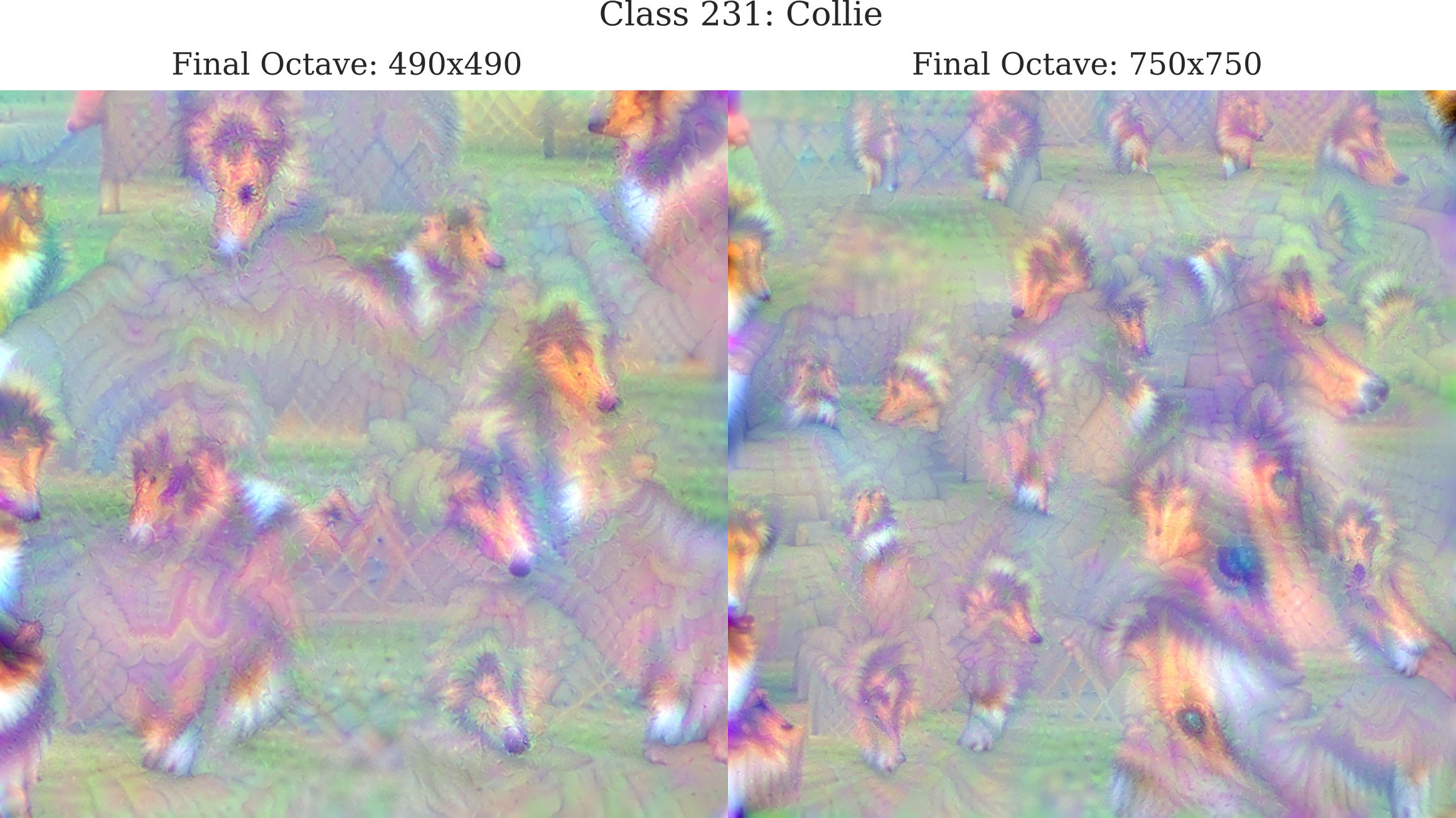
Earlier on this page it was noted that while the Octave method is able to make images that are far beyond the 299x299 resolution of the ImageNet training samples, there is a limit to how high a resolution one can hope to achieve because applying the gradient at different scales leads to incoherent images. This can be illustrated using the ResNet model fairly easily due to the high quality of the images this model generates. Observe how changing the last Octave to 750x750 (with a 720x720 crop size) while optimizing for ‘Collie’ leads to the appearance of the dog’s face at widely different scales in the bottom right, which leads to a somewhat more confusing if higher resolution image.
InceptionV3 and GoogleNet Compared
So far this page has documented a variety of different methods across two models that allow for the generation of a coherent (ie human-recognizable) input using gradient descent on an initial input of noise, with varying degrees of success. Measuring image coherence is somewhat difficult, as our metric is inherently subjective to the observer’s preference. Nevertheless, the octave method used with Googlenet has been observed to yield the most recognizable images thus far.
It may be wondered whether or not gradient descent using the same octaves would lead to similarly coherent images if applied to the InceptionV3 model, being that the choice of parameters, learning rates, and regularizers has optimized extensively for clarity whereas the octave approach for InceptionV3 documented above was not. Perhaps most importantly, more iterations were used and no L1 regularization was employed during gradient descent on the optimized octaves, as somewhat paradoxically L1 regularization on either the gradient or input led to an increase in noise. Using the optimized octave approach, images generated for all 1000 ImageNet classes using InceptionV3 can be compared to the images produced using GoogleNet.
It is worth investigating why inputs generated using GoogleNet are more coherent than those generated using InceptionV3, which is somewhat surprising being that InceptionV3 tends to be more accurate on ImageNet-based image identification challenges.
As a first step in this investigation, we can observe the process of input generation. Below are videos with each gradient descent iteration plotted over time, with a scatterplot of the activation values for each output class at that iteration on the right. First we have GoogleNet generating an input for target class ‘Stoplight’:
and now we have InceptionV3 generating an image for the same class, using the same optimization technique with octaves:
One can observe that the classification of InceptionV3 for its generated input is less stable from one iteration to the next than what is found for GoogleNet, particularly in the second octave. Resnet60 appears to be similar to GoogleNet with regards to activation stability.