Input Attribution and Adversarial Examples

Classification of Fashion MNIST images

The fashion MNIST dataset is a set of 28x28 monocolor images of articles of 10 types of clothing, labelled accordingly. Because these images are much smaller than the 256x256 pixel biological images above, the architectures used above must be modified (or else the input images must be reformatted to 256x256). The reason for this is because max pooling (or convolutions with no padding) lead to reductions in subsequent layer size, eventually resulting in a 0-dimensional layer. Thus the last four max pooling layers were removed from the deep network, and the last two from the AlexNet clone (code for these networks).

The deep network with no other modifications than noted above performs very well on the task of classifying the fashion MNIST dataset, and >91 % accuracy rate on test datasets achieved with no hyperparameter tuning.

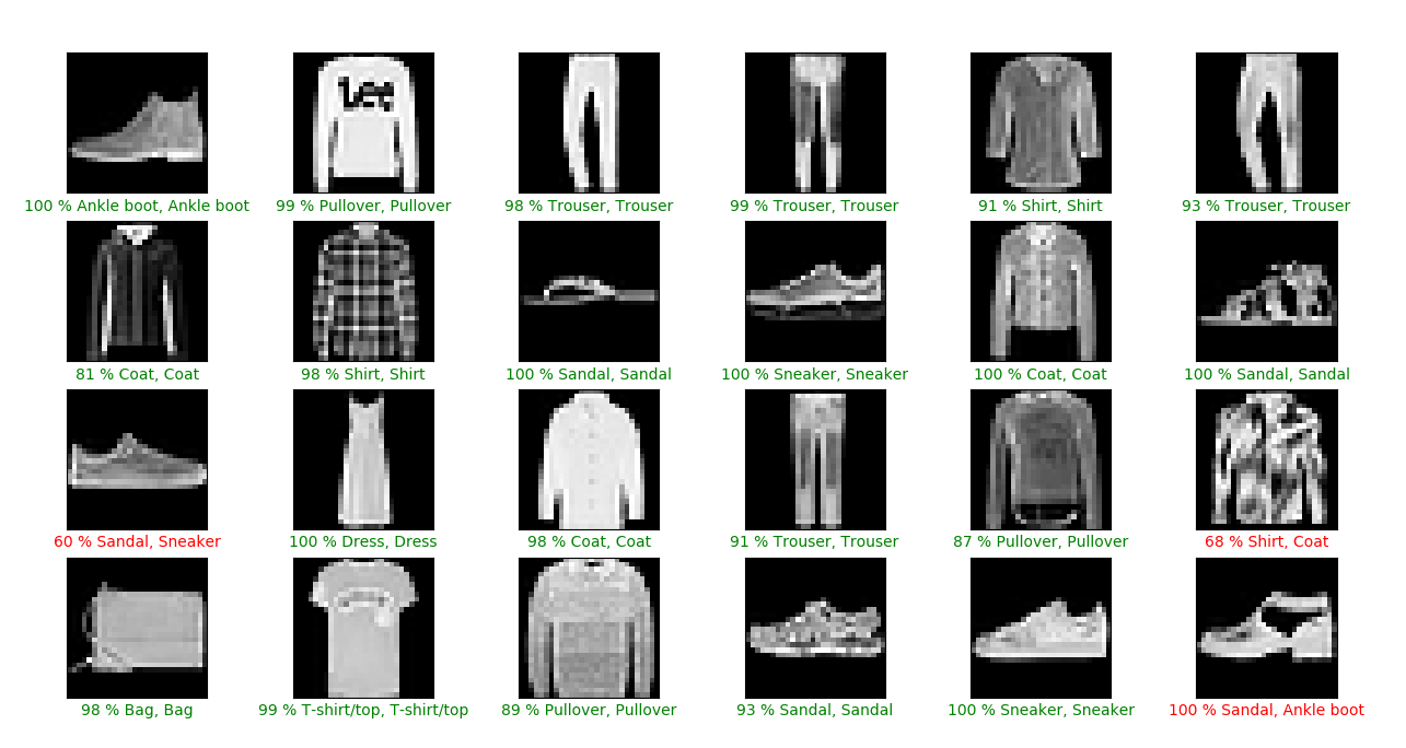
AlexNet achieves a ~72% accuracy rate on this dataset with no tuning or other modifications, although it trains much slower than the deep network as it has many more parameters (>10,000,000) than the deep network (~180,000).

We may observe a model’s attribution on the inputs from this dataset as well in order to understand how a trained model arrives at its conclusion. Here we have our standard model architecture and we compute the gradientxinput

\[\nabla_a O(a; \theta) * a\]

where the input $a$ is a tensor of the input image (28x28), the output of the model with parameters $\theta$ and input $a$ is $O(a; \theta)$, and $*$ denotes Hadamard (element-wise) multiplication. Here we implement gradientxinput using pytorch as follows:

def gradientxinput(model, input_tensor, output_dim):
	...
	input_tensor.requires_grad = True
	output = model.forward(input_tensor)
	output = output.reshape(1, output_dim).max()

	# backpropegate output gradient to input
	output.backward(retain_graph=True)
	gradientxinput = torch.abs(input_tensor.grad) * input_tensor
	return gradientxinput

Note that the figures below also have a max normalization step before returning the gradientxinput tensor. The gradientxinput object returned is a torch.Tensor() object and happily may be viewed directly using matplotlib.pyplot.imshow().

For an image of a sandal, we observe the following attribution:

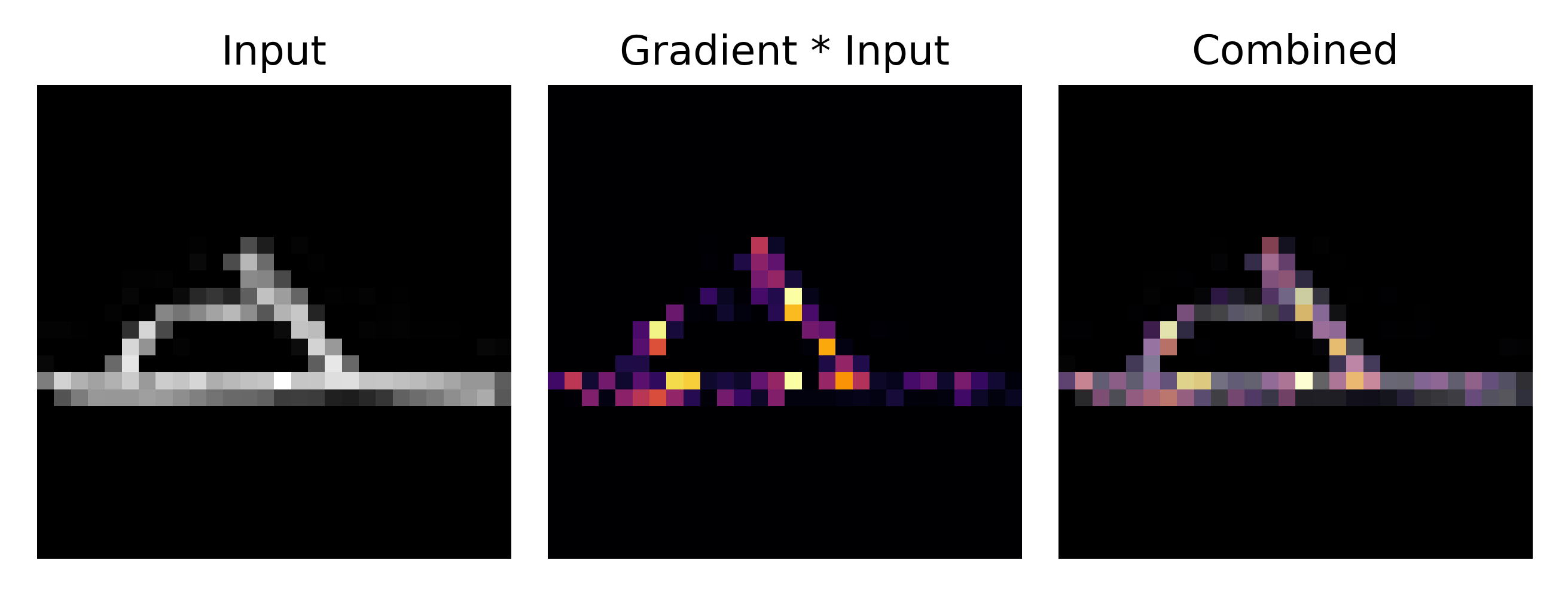
which focuses on certain points where the sandal top meets the sole. How does a deep learning model such as our convolutional network learn which regions of the input to focus on in order to minimize the cost function? At the start of training, there is a mostly random gradientxinput attribution for each image

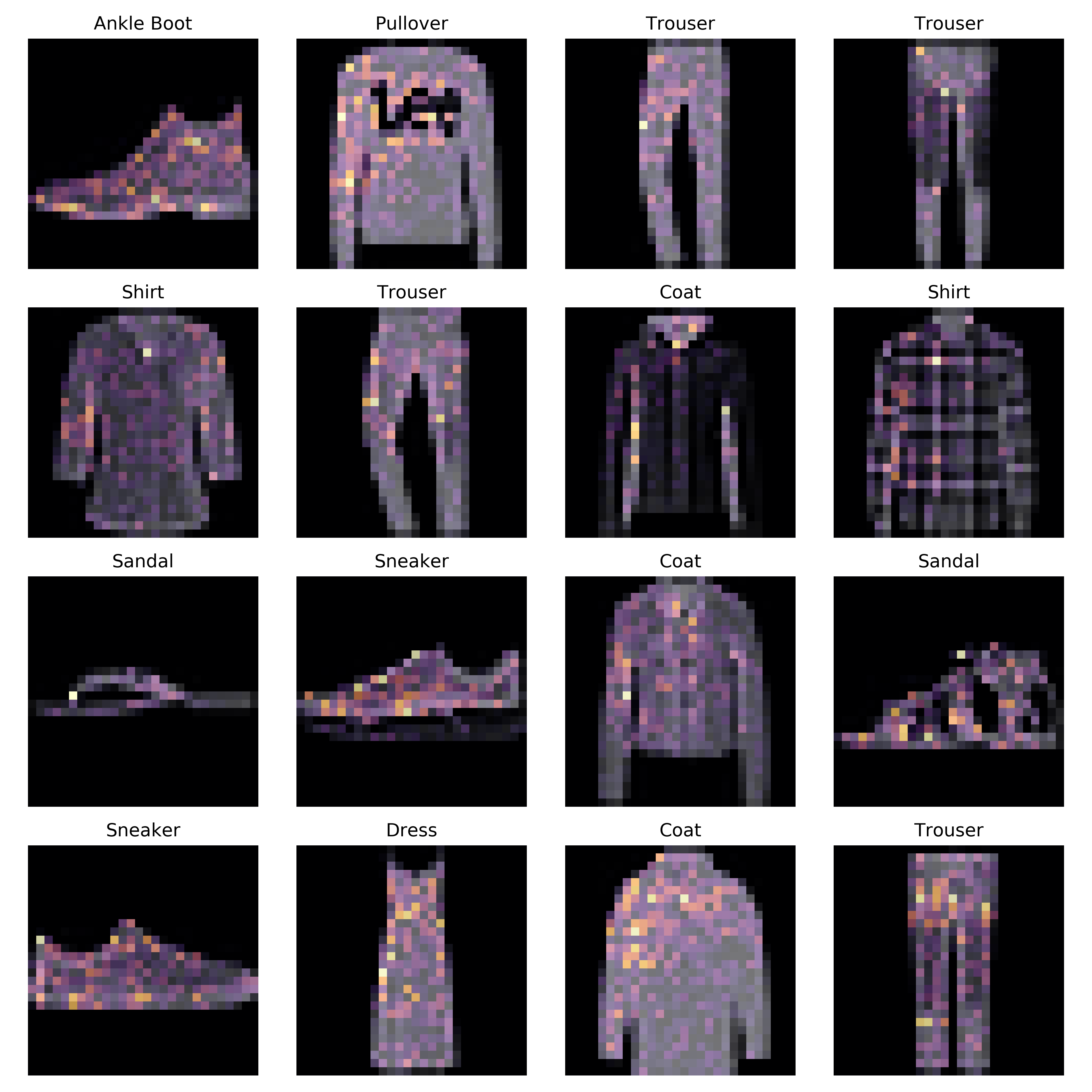
but at the end of training, certain stereotypical features of a given image category receive a larger attribution than others: for example, the elbows and collars of coats tend to exhibit a higher attribution than the rest of the garment.

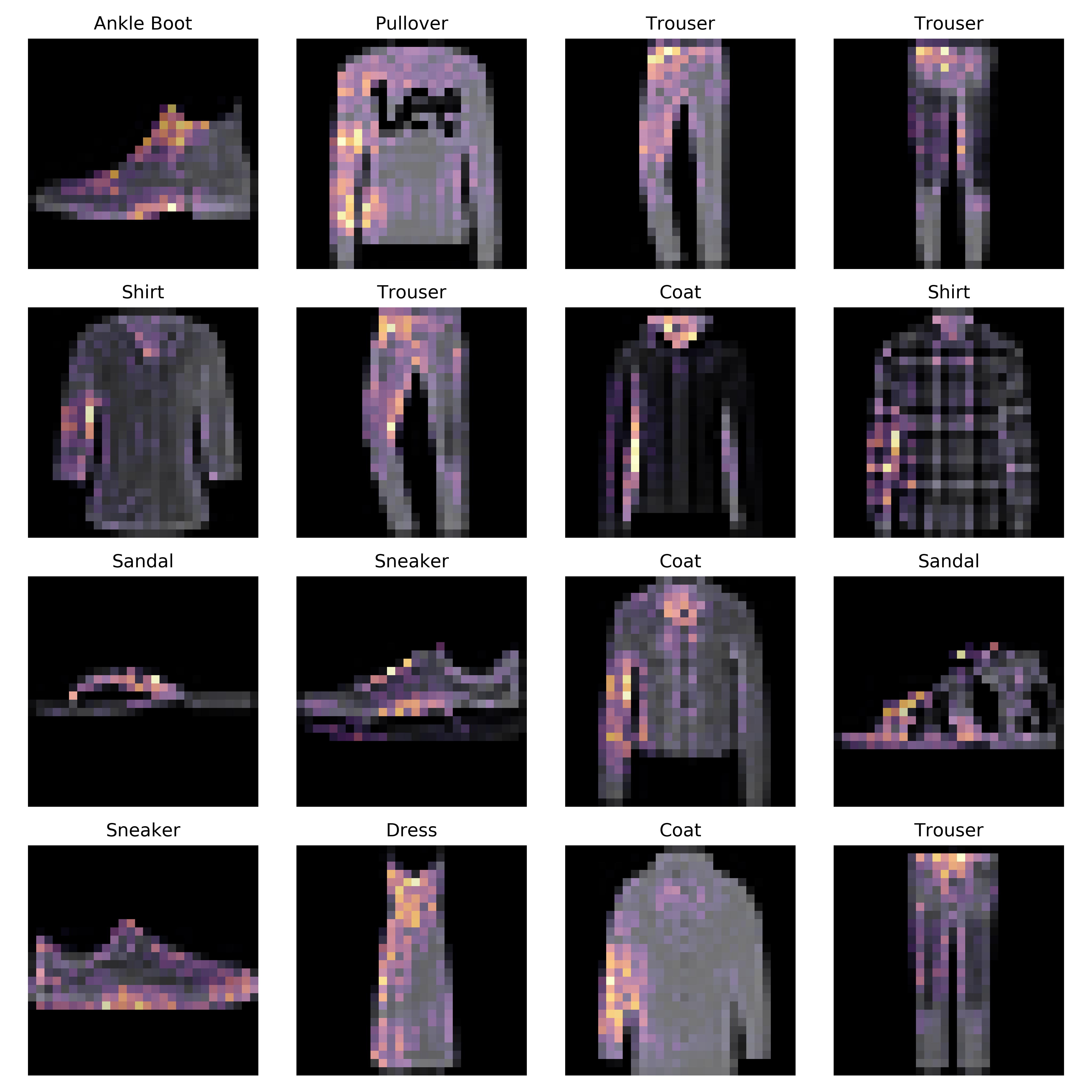
It is especially illuminating to observe how attribution changes after each minibatch gradient update. Here we go from the start of the start to the end of the training as show in the preceding images, plotting attributions on a subset of test set images after each minibatch (size 16) update.

Flower Type Identification

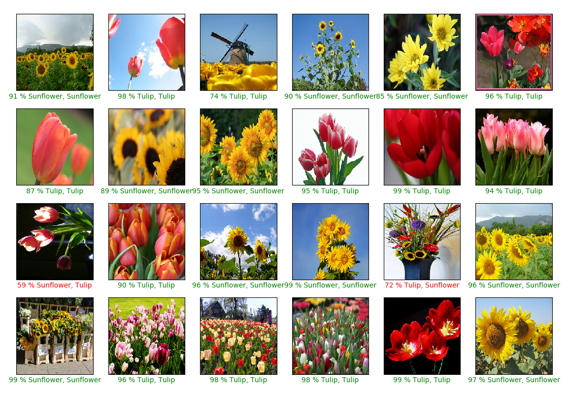
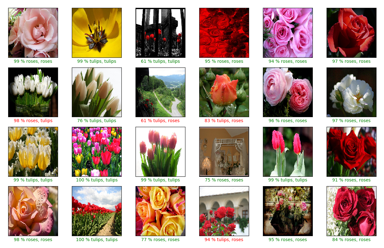
For some more colorful image classifications, lets turn to Alexander’s flower photoset, containing labeled images of sunflowers, tulips, dandelions, dasies, and roses. The deep network reaches a 61 % test classification score on this dataset, which increases to 91 % for binary discrimination between some flower types. Examples of this model classifying images of roses or dandelions,

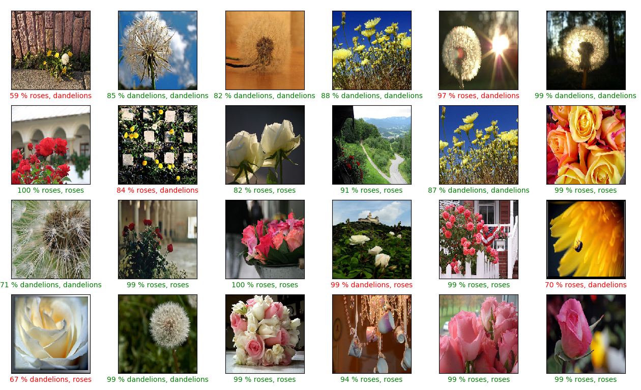
sunflowers or tulips,

and tulips or roses

We can investigate the learning process by using gradientxinput attribution. Before the start of training, we see that there is relatively random attribution placed on various pixels of test set flower images

but after 25 epochs, certain features are focused upon

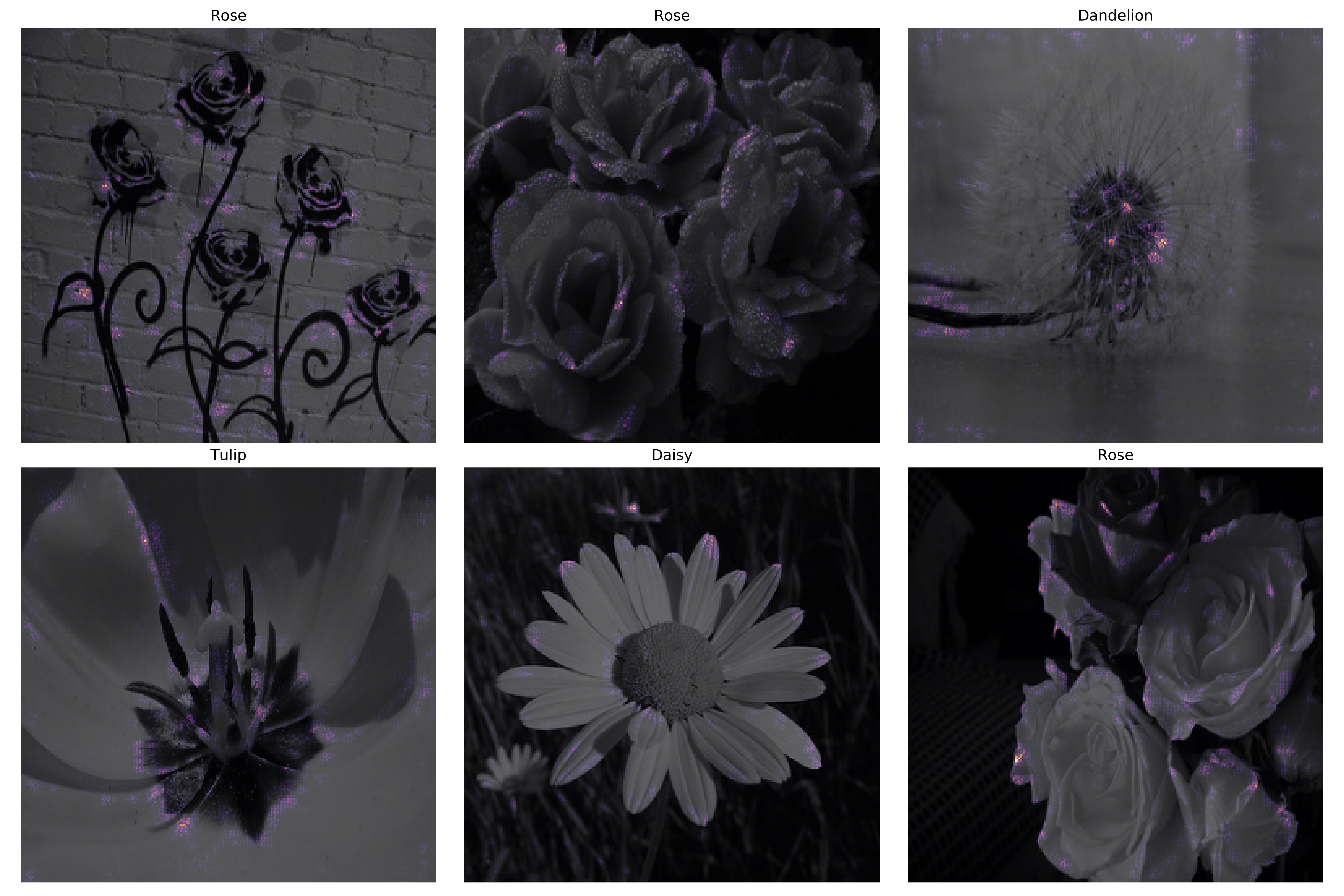
Plotting attribution after every minibatch update to the gradient, we have

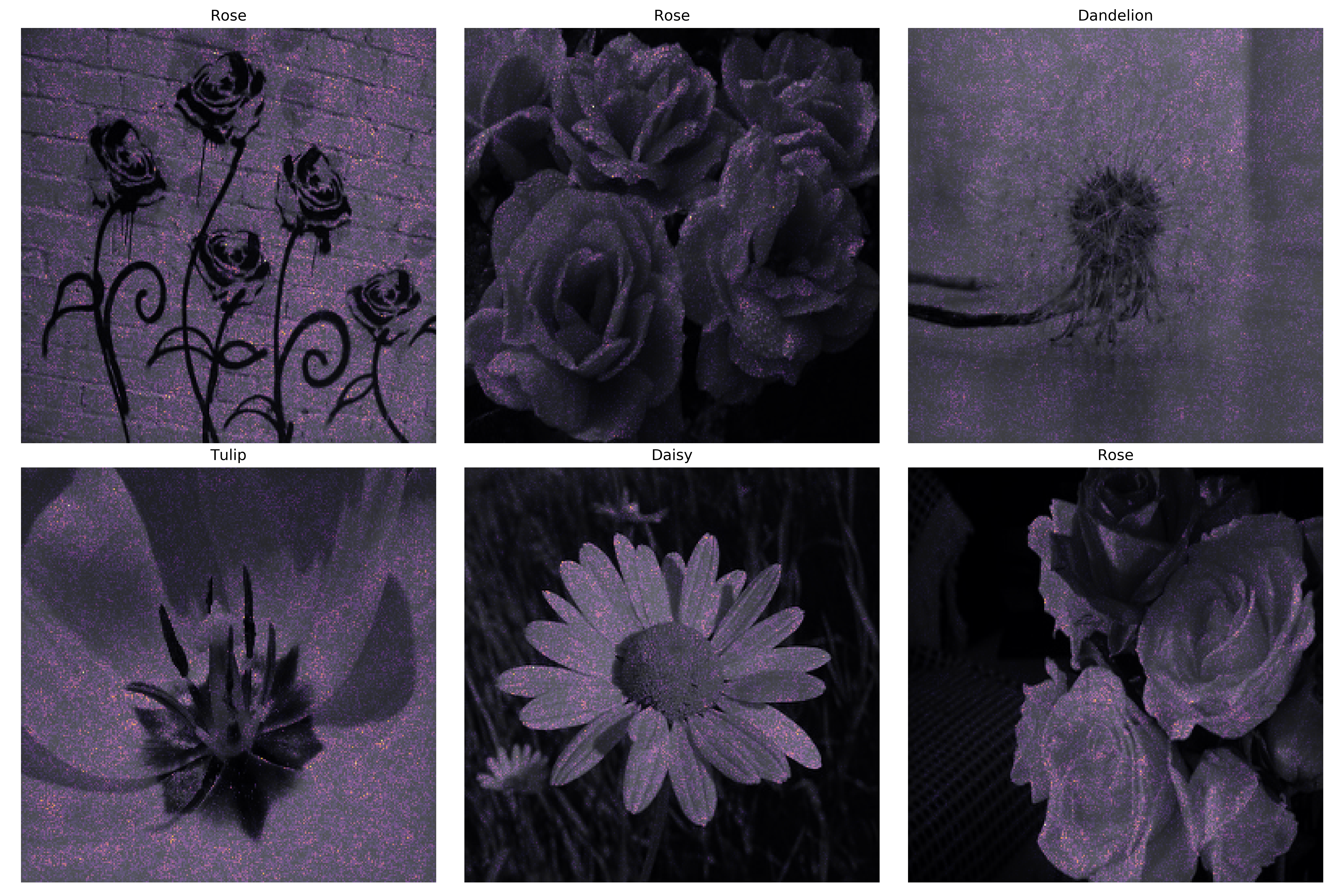
The deep learning models generally perform worse on flower type discrimination when they are not given color images, which makes sense being that flowers are usually quite colorful. Before the start of training, we have a stochastic attribution: note how the model places relatively high attribution on the sky in the bottom three images (especially the bottom right)

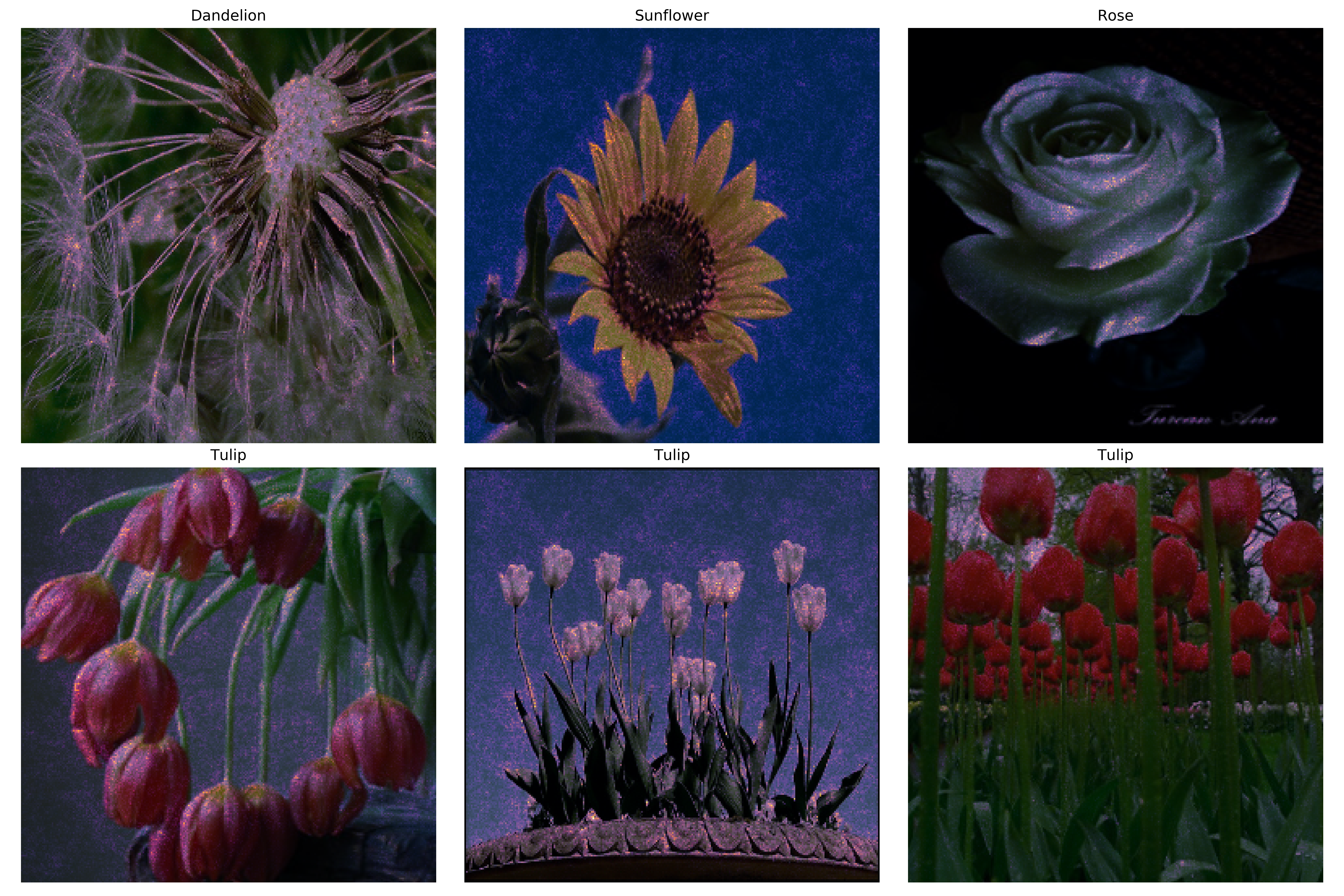
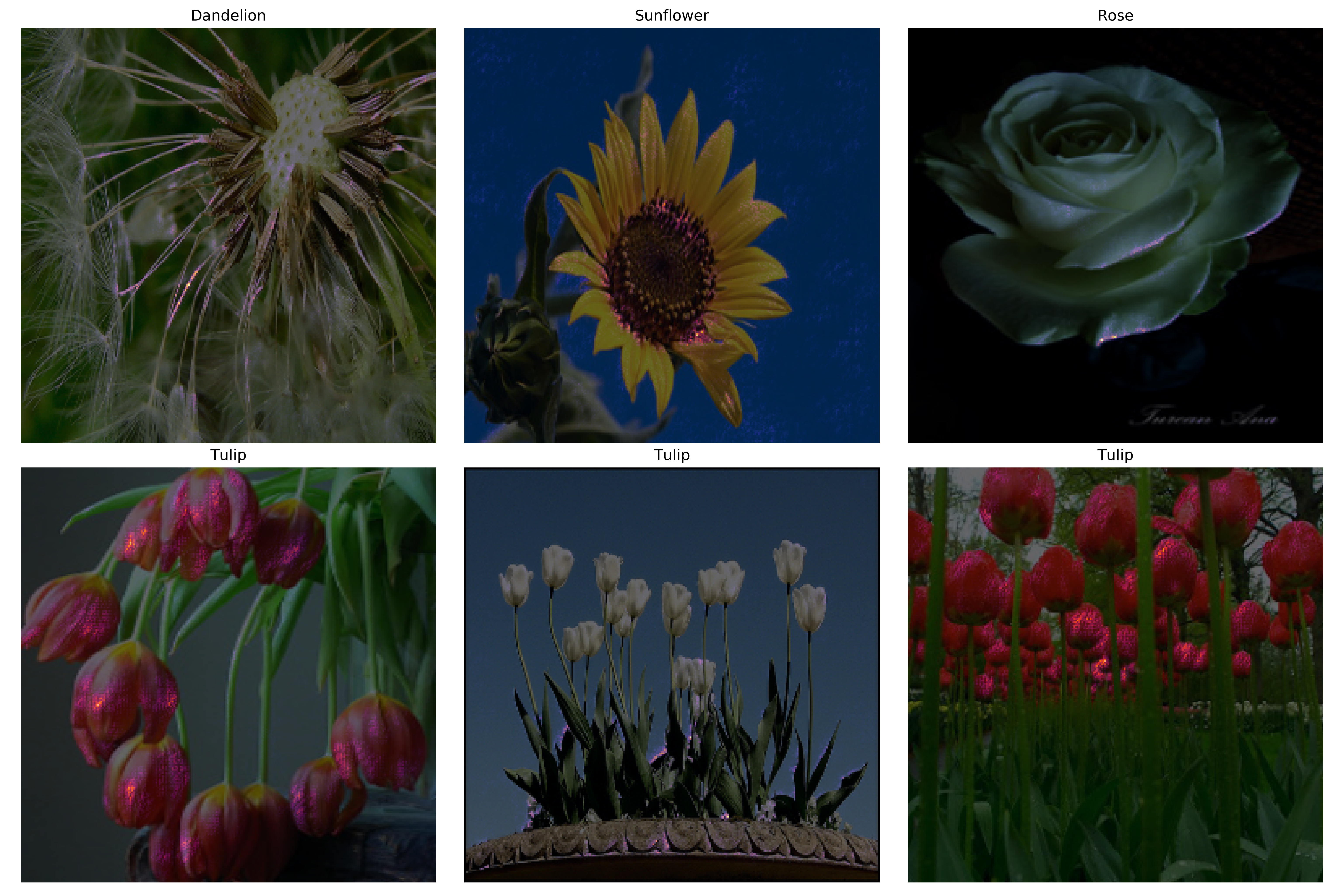
In contrast, after 25 epochs of training the model has learned to place more attribution on the tulip flower body, the edge of the rose petals, and the seeds of the sunflower and dandelion. Note that the bottom center tulip has questionable attribution: the edge of the leaves may be used to discriminate between plant types, but it is not likely that flower pot itself is a useful feature to focus on.

Plotting attribution after every minibatch update to the gradient, we have

Adversarial Examples

Considering the attribution patterns placed on various input images, it may seem that a deep learning object recognition process is similar to a human-like decision making process when identifying images: focus on the features that differ between images and learn which features correspond to what image. But there are significant differences between natural and deep learning-based object recognition, and one of the most dramatic of these differences is the presence of what has been termed ‘adversarial examples’, first observed by Szegedy and colleagues in their paper on this subject.

To those of you who have read this page on the subject, the presence of adversarial examples should come as no surprise: as a model becomes able to discriminate between more and more input images it better and better approximates a one-to-one mapping between a multidimensional input (the image) and a one-dimensional output (the cost function). To summarize the argument on that page, there are no continuous one-to-one (bijective) mappings possible from two or more dimensions to one, we would expect to see discontinuities in a function approximating a bijective map between many and one dimension. This is precisely what occurs when an image tensor input (which for a 28x28 image is 784-dimensional) is mapped by a deep learning model to a loss value by $J(O(a; \theta), y)$.

How might we go about finding an adversarial example? One option is to compute the gradient $g$ of the loss function of the output $J(O)$ with respect to the input $a$ of the model with parameters $\theta$ with a true classification $y$,

\[g = \nabla_a J(O(a; \theta), y)\]

but instead of taking a small step against the gradient (as would be the case if we were computing $\nabla_{\theta} J(O(a; \theta))$ and then taking a small step in the opposite direction during stochastic gradient descent), we first find the direction along each input tensor element that $g$ projects onto with $\mathrm{sign}(g)$ and then take a small step in this direction.

\[a' = a + \epsilon * \mathrm{sign}(g)\]

where the $\mathrm{sign}()$ function the real-valued elements of a tensor $a$ to either 1 or -1, or more precisely this function

\[f: \Bbb R \to \{ -1, 1 \}\]

depending on the sign of each element $a_n \in a$. This is known as the fast gradient sign method, and has been reported to yield adversarial examples for practically any CIFAR image dataset input when applied to a trained AlexNet architecture.

What this procedure accomplishes is to change the input by a small amount (determined by the size of $\epsilon$) in the direction that makes the cost function $J$ increase the most, which intuitively is effectively the same as making the input a slightly different in precisely the direction per pixel that makes the neural network less accurate.

To implement this, first we need to calculate $g$, which may be accomplished as follows:

def loss_gradient(model, input_tensor, true_output, output_dim):
	... # see source code for the full method with documentation
	true_output = true_output.reshape(1)
	input_tensor.requires_grad = True
	output = model.forward(input_tensor)
	loss = loss_fn(output, true_output) # objective function applied (negative log likelihood)

	# only scalars may be assigned a gradient
	output = output.reshape(1, output_dim).max()

	# backpropegate output gradient to input
	loss.backward(retain_graph=True)
	gradient = input_tensor.grad
	return gradient

Now we need to calculate $a’$, and here we assign $\epsilon=0.01$. Next we find the model’s output for $a$ as well as $a’$, and throw in an output for $g$ for good measure

def generate_adversaries(model, input_tensors, output_tensors, index):
	... # see source code for the full method with documentation
	single_input= input_tensors[index].reshape(1, 3, 256, 256)
	input_grad = torch.sign(loss_gradient(model, single_input, output_tensors[index], 5))
	added_input = single_input + 0.01*input_grad
	
	original_pred = model(single_input)
	grad_pred = model(0.01*input_grad)
	adversarial_pred = model(added_input)

Now we can plot images of $a$ and the output of each fed to the model by reshaping the tensor for use in plt.imshow() before finding the output class and output confidence (as we are using a softmax output) from $O(a; \theta)$ as follows

	...
	input_img = single_input.reshape(3, 256, 256).permute(1, 2, 0).detach().numpy() # reshape for imshow 
	original_class = class_names[int(original_pred.argmax(1))].title() # find output class
	original_confidence = int(max(original_pred.detach().numpy()[0]) * 100) # find output confidence w/softmax output

and finally we can perform the same procedure to yield $g$ and $a’$.

For an untrained model with randomized $\theta$, $O(a’;\theta)$ is generally quite similar to $O(a;\theta)$. The figures below display typical results from computing $\mathrm{sign}(g)$ (center) from the original input $a$ (left) with the modified input $a’$ (right). Note that the image representation of the sign of the gradient clips negative values (black pixels in the image) and is not a true representation of what is actually added to $a$: the true image of $\mathrm{sign}(g)$ is 50 times dimmer than shown because by design $\epsilon * \mathrm{sign}(g)$ is practically invisible. The model’s output for $a$ and $a’$ is noted above the image, with the softmax value converted to a percentage for clarity.

After training, however, we see some dramatic changes in the model’s output (and ability to classify) the image $a$ compared to the shifted image $a’$. In the following three examples, the model’s classification for $a$ is accurate, but the addition of an imperceptably small amount of the middle image to make $a’$ yields a confident but incorrect classification.

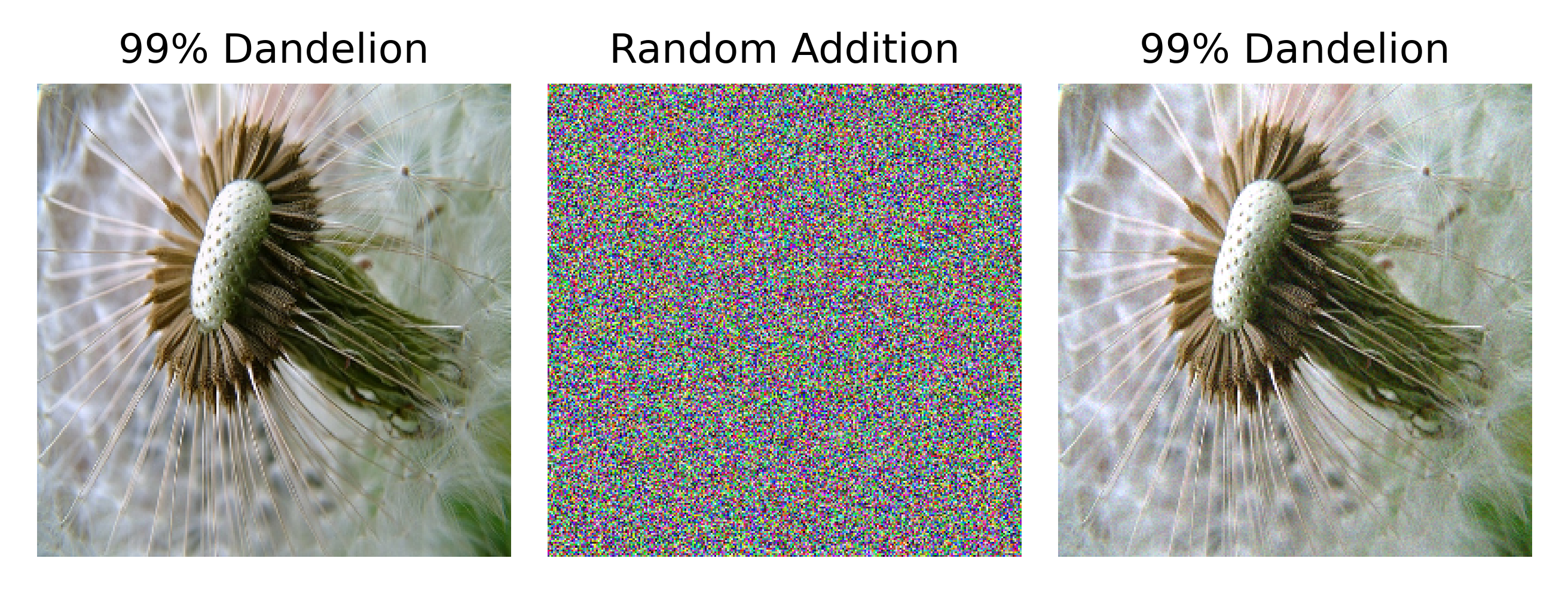
In contrast, the addition of pixels that are randomly assigned only rarely changes the model’s output significantly. The following is a typical example of the result of addition of a random tensor to a given input image.

Not all shifted images experience this change in predicted classification: the following images are viewed virtually identically by the model. After 40 epochs of training a cNN, around a third of all inputs follow this pattern such that the model does not change its output significantly when given $a’$ as an input instead of $a$ for $\epsilon=0.01$. Note that increasing the value of $\epsilon$ leads to nearly every input image having an adversarial example using the fast gradient sign method, even if the images are still not noticeably different.

It is interesting to note that the gradient sign image itself may be confidently (and necessarily incorrectly) classified too.

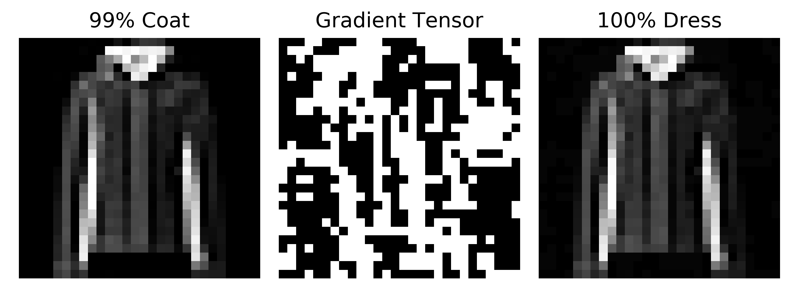
Can we find adversarial examples for simpler inputs as well as complicated ones? Indeed we can: after applying the gradient step method to 28x28 pixel Fashion MNIST images using a model trained to classify these inputs, we can find adversarial examples just as we saw for flowers.

It may see strange to take the sign of the gradient per pixel rather than the projection of the gradient itself, as would be the case if $a$ were a trainable parameter during gradient descent. The authors this work made this decision in order to emphasize the ability of a linear transformation in the input to create adversarial examples, and went on to assert that the major cause of adversarial examples in general is excessive linearity in deep learning models.

It is probable that such linearity does indeed make finding adversarial examples somewhat easier, but if the argument on this page is accepted then attempting to prevent adversarial examples using nonlinear activation functions or specialized architectures is bound to fail, as all $f: \Bbb R^n \to \Bbb R$ are discontinuous if bijective. Not only that, but such $f$ are everywhere discontinuous, which is why each input image will have an adversarial example if we assume that $f$ approximates a bijective function well enough.

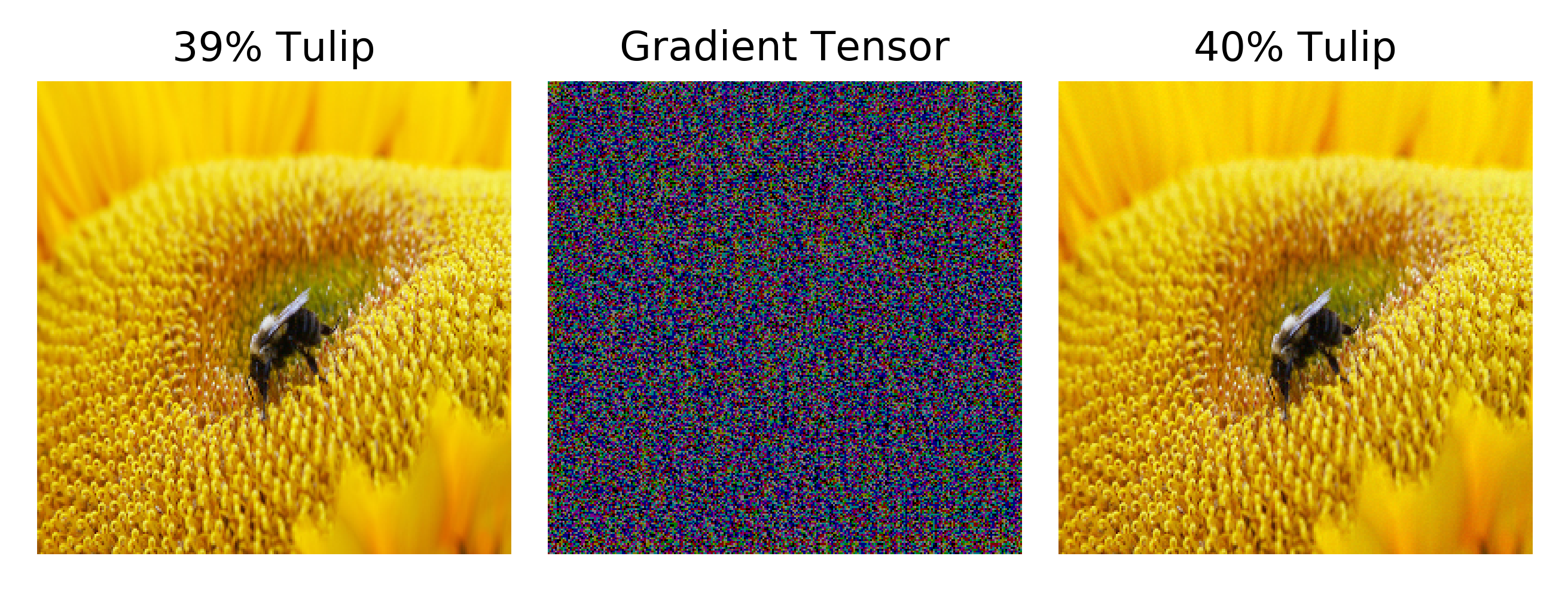
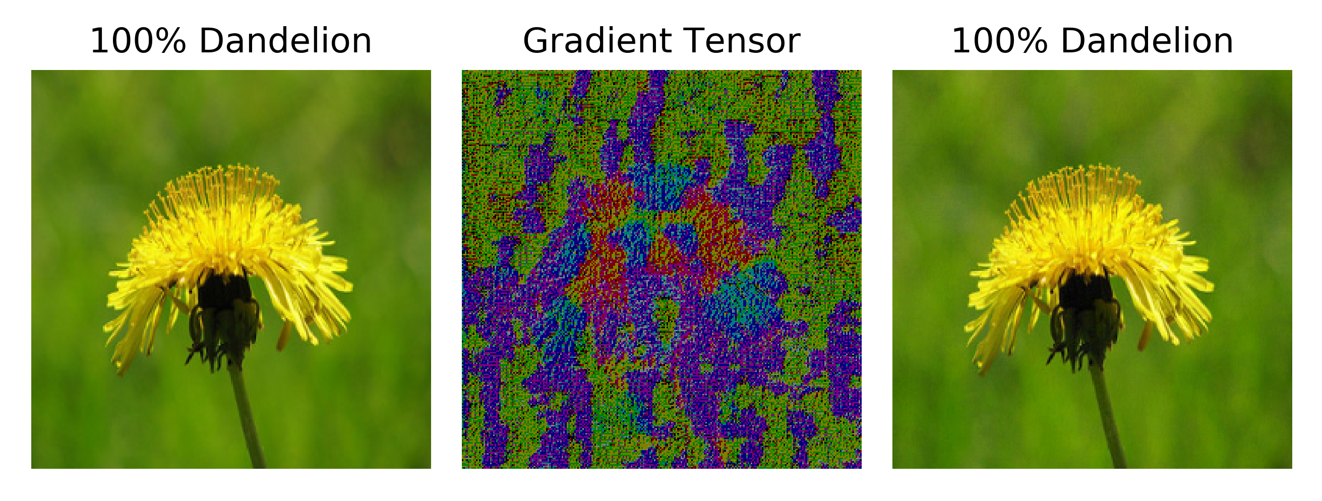
What happens when we manipulate the image according to the gradient of the objective function, rather than its sign? Geometrically this signifies taking the projection of the gradient $g$

\[g = \nabla_a J(O(a; \theta), y)\]

onto each input element $a_n$, which tells us not only which pixels to modify but also how much to modify them. When we scale this gradient by max norming

\[g' = \frac{g}{\mathrm{max} (g)}\]

and then applying this normed gradient to the input $a$ to make $a’$

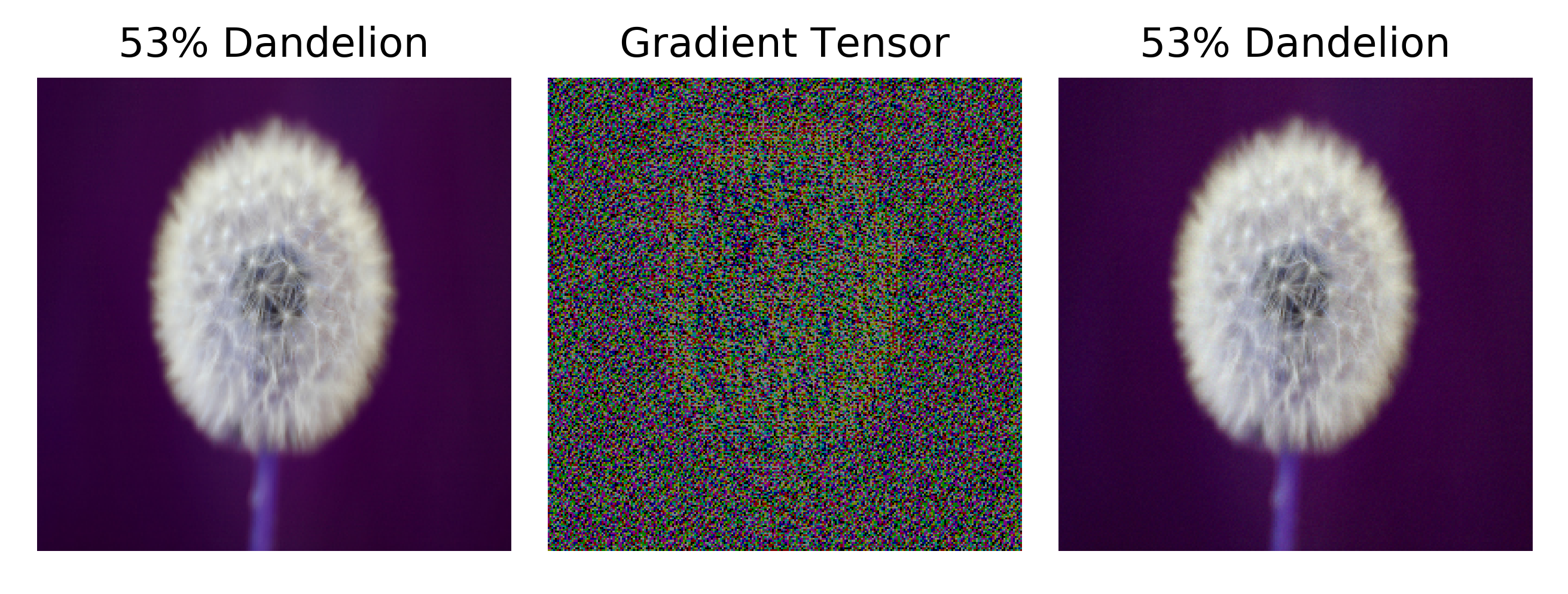
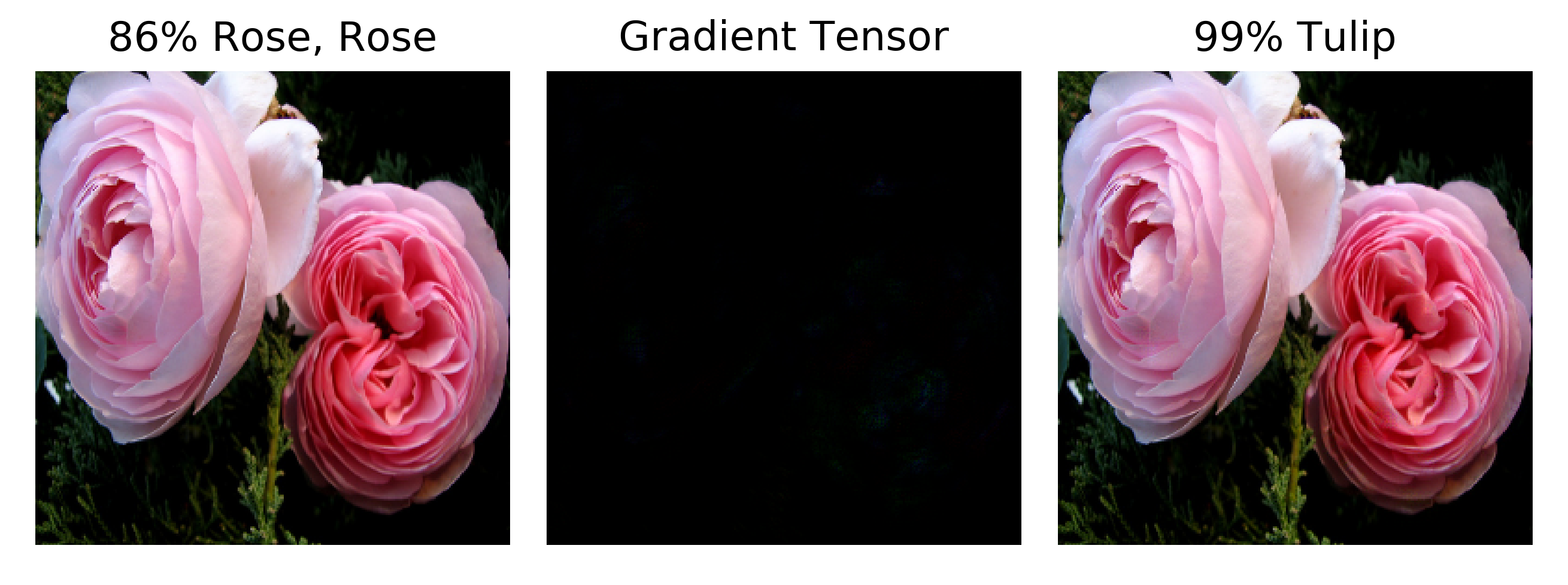
\[a' = a + \epsilon * g'\]

we once again find adversarial examples, even with very small $\epsilon$. Here the gradient tensor image is to scale: the center image is $\epsilon *g’$ and has values that are not scaled up as they were in the other images on this page (and the prediction for $a$ on the left is followed by the true classification for clarity)

Empirically this method performs as well if not better than the fast gradient sign procedure with respect to adversarial example generation: while keeping $\epsilon$ small enough to be unnoticeable, the majority of inputs may be found to have corresponding adversarial examples.

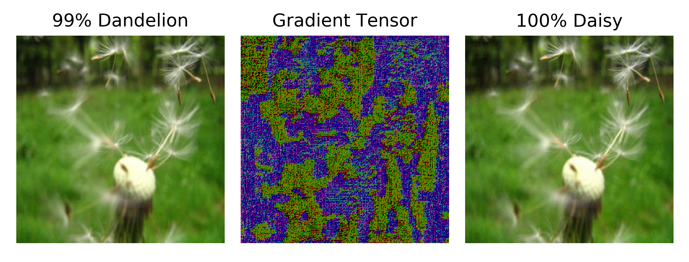
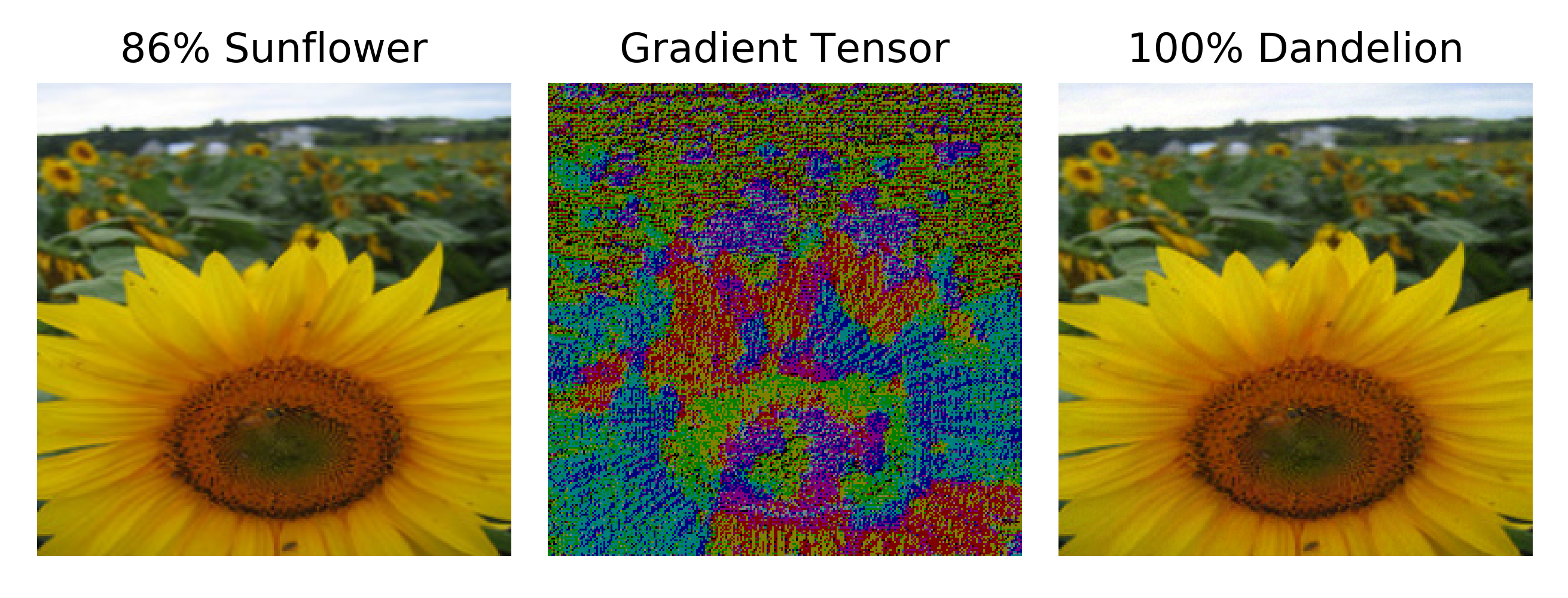
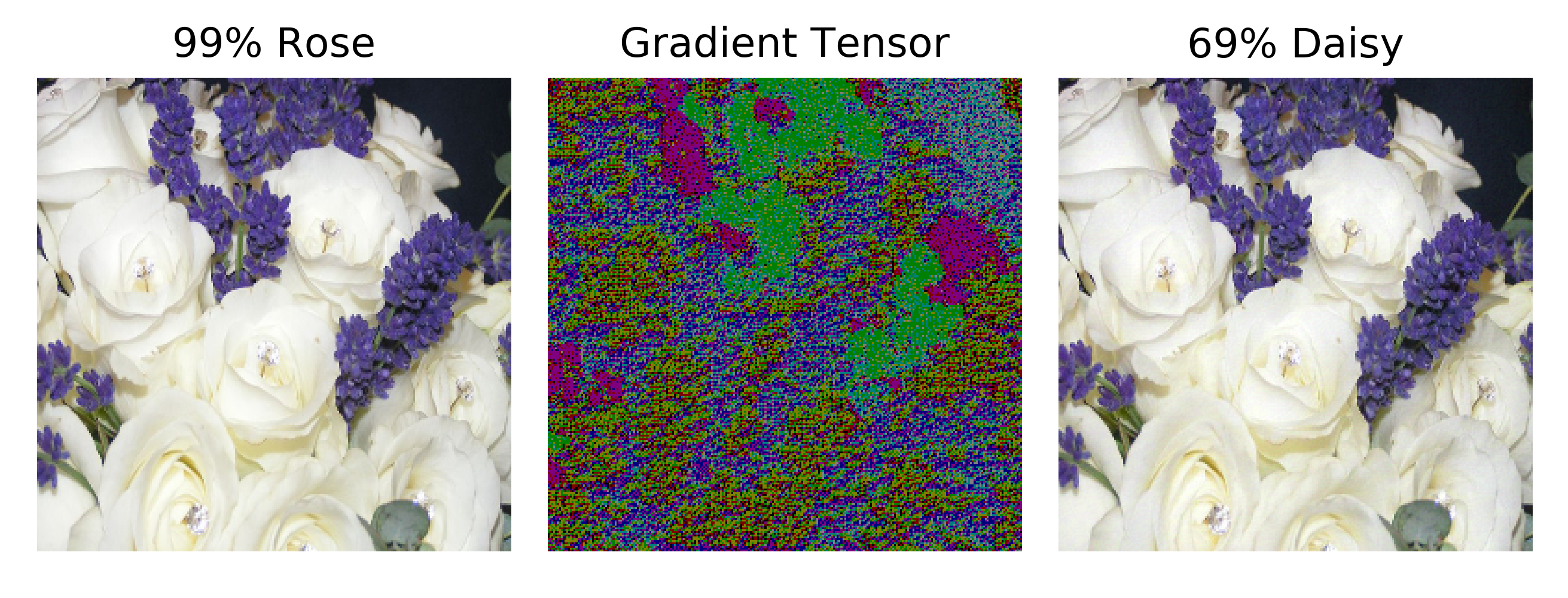
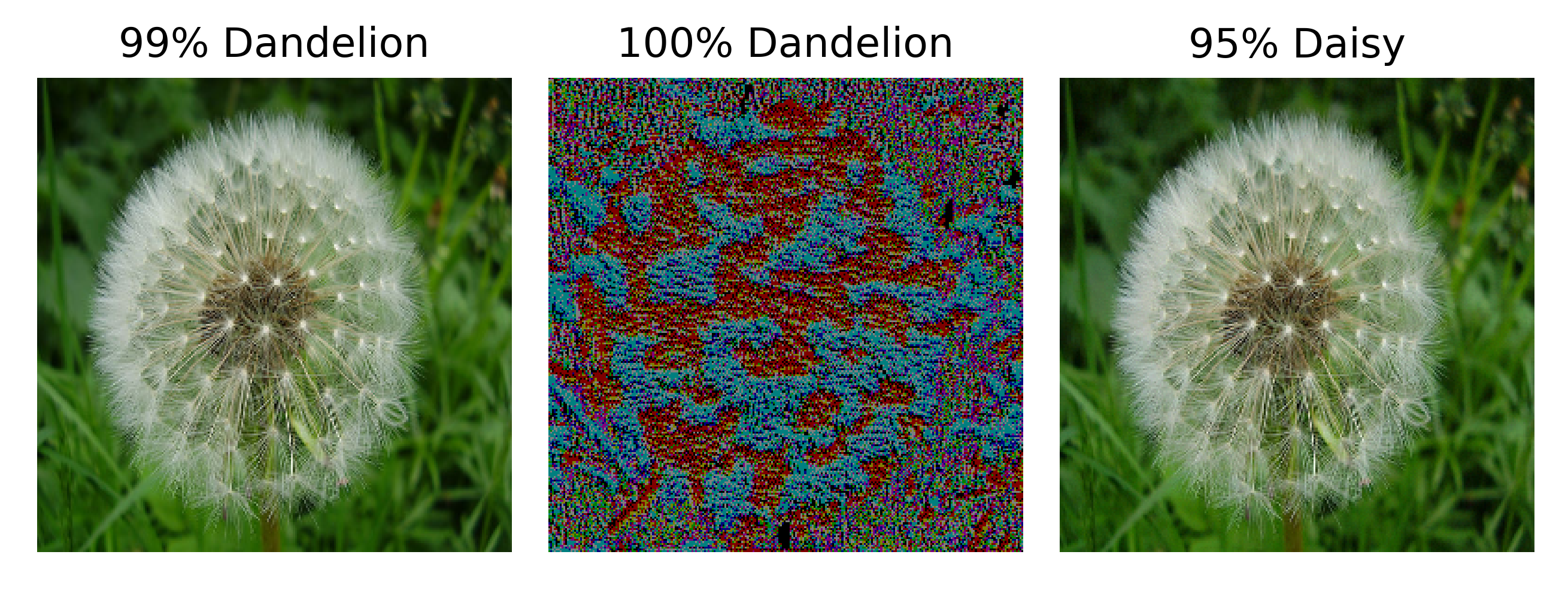
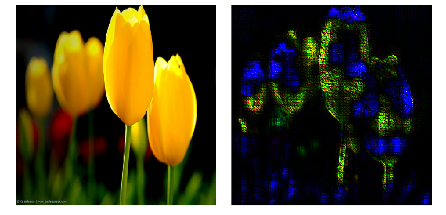
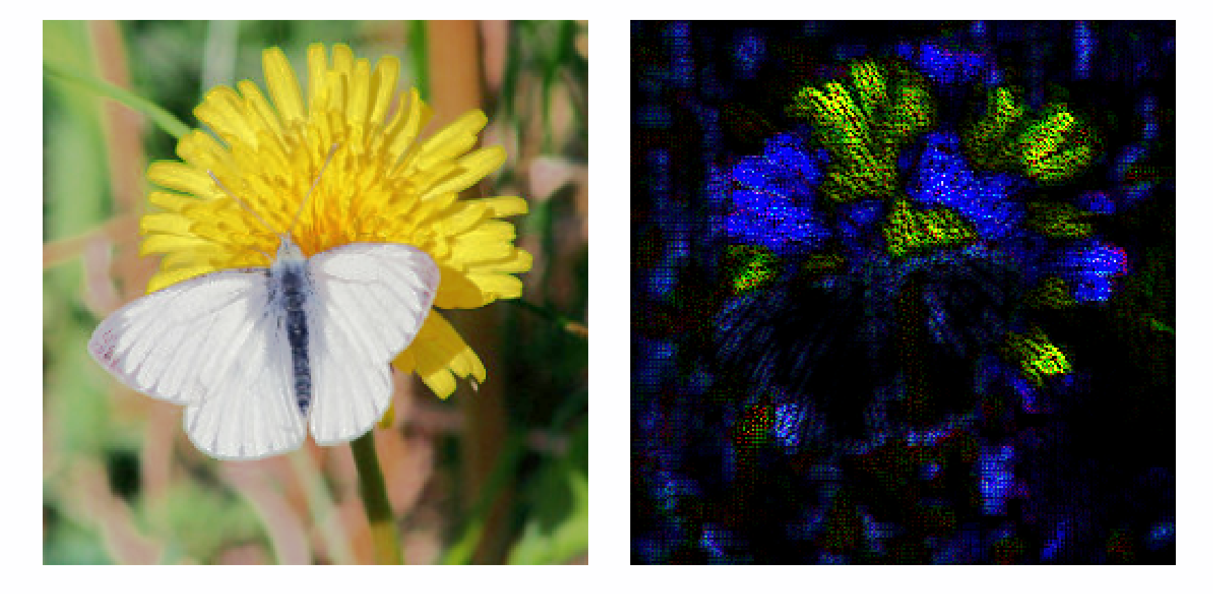
It is interesting to observe the gradient images in more detail: here we have the continuous gradient $\epsilon * g’$ scaled to be 60 times brighter (ie larger values) than $\epsilon * g’$ for clarity.

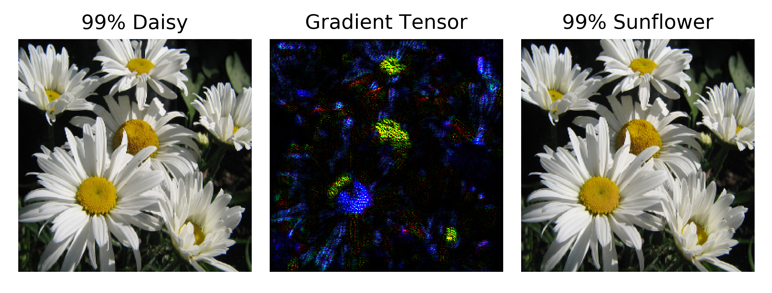
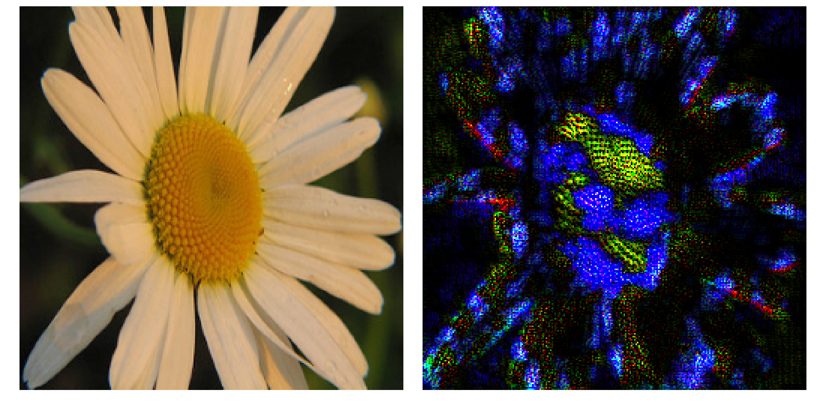
Close inspection of the image of $\epsilon * g’$ reveals something interesting: the gradient tensor appears to mirror a number of the features of the original input image, except with dark blue petals instead of white and a mix of blue and yellow where the disk flourets (center yellow parts) are found in the original image. This may be thought of as a recapitulation of the features of an input image itself from the sole informational content of the gradient of the loss function with respect to the input,

\[\nabla_a J(O(a; \theta), y)\]

Recalling how forward propegation followed by backpropegation is used in order to compute this gradient, we find that these features remain after nearly two dozen vector arithmetic operations, none of which are necessarily feature-preserving. From an informational perspective, one can think of this as the information from the input being fed into the neural network, stored as activations in the network’s various layers, before that information is then used to find the gradient of the loss function with respect to the input.

The above image is not the only input that has features that are recapitulated in the input gradient: here some tulips

and a butterfly on a dandelion

and the same is found for a daisy.

It is important to note that untrained models are incapable of preserving practically any input features in the input gradient. This is to be expected given that the component operations of forward and backpropegation have no guarantee to preserve any information.

Additive Attributions for Nonlocality

In the last section, we saw that the training process (here 40 epochs) leads to a preservation of certain features of the input image in the gradient of the input with respect to the loss function. We can observe the process of feature preservation during model training as follows:

Gradientxinput has been criticized for relying entirely on locality: the gradient of a point in multidimensional space is only accurate in an infinitesmal region around that point by definition. Practically this means that if an input were to change substantially, a pure gradient-based input attribution method may not be able to correctly attribute that change to the output (or loss function) if there is not a local-to-global equivalence in the model in question.

There are a number of ways to ameliorate this problem. One is to directly interfere with (occlude) the input, usually in some fairly large way before observing the effect on the output. For image data, this could mean zeroing out all pixels in a given region that scans over the entire input. For sequential data as seen here, successive characters can be modified as the model output is observed. Occlusion usually introduces substantial changes from the original input meaning that the observed output changes are not the result of local changes. Occlusion can be combined with gradientxinput to make a fairly robust attribution method.

Another way to address locality is to add up gradients as the input is formed in a straight-line path from some null reference, an approach put forward in this paper by Yan and colleages. More concretely, a blank image may serve as a null reference and the true image may be formed by increasing brightness (our straight-line path) until the true image is recovered. At certain points along this process, the gradients of the model with respect to the input may be added to make one integrated gradient measurment. This method has some benefits but also has a significant downside: for many types of input, there is no clear straight-line path. Image input data has a couple clear paths (brightness and contrast) but discrete inputs such as language encodings do not.

An alternative to this approach could be to integrate input gradients but instead of varying inputs for a trained network, we integrate the input gradients during training for one given input $a$. If we were to use the loss gradient, for each configuration $\theta_n$ of the model during training we have

\[g = \sum_{n} \nabla_a J(O(a; \theta_n), y)\]

This method may be used for any input type, regardless of an ability to transform from a baseline.