Language Modeling and Discrete Encodings
This page is a continuation of Parts I and II.
Introduction
In Part II it was observed that hidden layer representations of the model input are typically hopelessly inaccurate, which is somewhat surprising being that vision transformers and convolutional models are capable of quite accurate input representation even in deeper layers. This page begins by further testing representation accuracy before exploring the theory behind input representation accuracy for language models, and theory as to why this accuracy is important to language modeling tasks.
Restricted Vocabulary Input Representation
Why are trained GPT-2 models incapable of accurate input representation? Observing the spatial pattern of feature and input representations (see here for work on this topic) gives us a hypothesis: in that work it is apparent that trained GPT-2 transformer blocks introduce high-frequency noise into the input representation of two images such that the argument maximum value of all pixels is no longer meaningful. On this page we deal with the argmax of logits which are transformed via a Moore-Penrose pseudoinverse, but it stands to reason that a similar phenomenon is occuring here such that the argmax of the logits becomes unpredictable due to the introduction of high-frequency noise in $a_g$.
One way to test this idea is to note that the vast majority of the $50257$ tokens present in the GPT-2 vocabulary signify words or word parts that are extremely unlikely to be observed in real text. Indeed it appears that these very tokens are the ones that tend to result when the $\mathrm{arg \; max}$ function is called on the logits of those token indicies for trained GPT-2.
To prevent high-valued but rare tokens from being selected during the decoding process, we can simply mask all the tokens that are not selected (not in the allowed_tokens tensor) with 0 and proceed with argmax as before.
def masked_decode(logits: torch.tensor, allowed_tokens: torch.tensor) -> str:
	mask_tensor = torch.zeros(logits.shape).to(device)
	mask_tensor[:, :, allowed_tokens] = 1.
	masked_logits = logits * mask_tensor
	allowed_output = torch.argmax(masked_logits, dim=2)[0]
	output = tokenizer.decode(allowed_output)

	return output
If we are very selective with our allowed_tokens and only allow words in the target input to be selected, we find that the input may be exactly recovered by a trained GPT-2 transformer block, such that the input representation is for $N=2000$ is $a_g = \mathrm{The \; sky \; is \; blue.}$ With some learning rate tuning and a sufficiently large $N$, we can recover the target input even for 4 transformer blocks, but for all 12 blocks it is rare that $a_g = a$ even after tuning such that $\vert \vert a_g - a \vert \vert < \vert \vert a’ - a \vert \vert$.
This is remarkable in that even a very small expansion of the allowed vocabulary results in a trained GPT-2 block being unable to accurately recognize the input. For example, given the words of the sentence ‘The sky is blue or red depending on the time of day.’ as our allowed tokens, after $N=20k$ steps we have
\[a_g = \mathtt{\; day \; or \; day \; blue \; or}\]In contrast, the same model before training is capable of recovering the target input after $N=200$ steps. Note that neither trained nor untrained GPT-2 model with all 12 blocks is capable of recovering the input for even that slightly expanded vocabulary.
Direct Input Representation
Early on this page, two methods to deal with the discrete nature of language inputs were noted: the first was to simply ignore them during the gradient descent process and convert the outputs back to tokens via the Moore-Penrose pseudoinverse, and this is arguably the most natural choice as it involves the fewest changes to the model itself. Another option is to transform the input tokens (an array of integers) into a vector space and perform gradient descent directly with that space being the terminal node of the backpropegation computational graph.
To be precise, what we want is to convert an array of input tokens $a_t$, which for example could be
\[a_t = [1, 0, 2]\]to continuous values in a vector space, which for the above example could be
\[a = \begin{bmatrix} 0 & 1. & 0 \\ 1. & 0 & 0 \\ 0 & 0 & 1. \\ \end{bmatrix}\]but note that there is no specific rule for converting a token to a vector value, for instance we could instead assign any small value as a baseline with a larger value as the corresponding indicies. For GPT-2, we can find what the trained embedding assigns for each input element by finding the Moore-Pensore pseudoinverse of the weight matrix of the embedding, denoted $W^+$, as follows:
\[a = W^+E(a_t)\]where $a_t$ corresponds to an array of integers and $E$ signifies the embedding transformation that maps these integers to an embedding vector space.
which can be implemented as
embedding = model.transformer.wte(tokens)
embedding_weight = model.transformer.wte.weight.float() # convert to float in case model is in 16-bit precision
inverse_embedding = torch.linalg.pinv(embedding_weight)
logits = torch.matmul(embedding, inverse_embedding) # invert embedding transformations
Verifying that this procedure is accurate is not too hard, and may be done by first converting the vector space back to integer tokens via the $\mathrm{arg \; max}$ of each logit, and then decoding this array of integers as shown below.
tokens = torch.argmax(target_logits, dim=2)[0]
output = tokenizer.decode(tokens)
With this procedure, we find that the trained GPT-2 word-token embedding maps the value at the index of the integer token to a value on the order of $1 \times 10^{-2}$ whereas the values of other indices are typically $\leq 1 \times 10^{-3}$. We can also simply mandate that the vector values at indicies corresponding to the appropriate tokens have some large positive value and that all others are zero as follows:
target_logits = torch.zeros(logits.shape).to(device)
for i in range(len(tokens[0])):
	target_logits[:, i, tokens[0, i]] = 10
There does not appear to be any significant difference between these two approaches to mapping $a_t \to a$.
Now that we have a continuous $a$ input, we can perform gradient descent on the model’s output as follows:
\[a_{n+1} = a_n + \eta * \nabla_{a_n} ||O_l(a_n, \theta) - O_l(a, \theta)||_1 \\ \tag{5}\label{eq5}\]where $a_0 = \mathcal N(a, \mu=1/2, \sigma=1/20)$. The GPT-2 model also needs to be modified as the word-to-embedding transformation is designed to take in integer ‘words’ rather than vectors, and this can be ameliorated by replacing this transformation with a multiplication of the input by the word-to-embedding transformation weights as follows.
class InputGPT(nn.Module):

	def __init__(self, model):
		super().__init__()
		self.model = model

	def forward(self, x: torch.tensor) -> torch.tensor:
		# replaces wte transformation
		x = torch.matmul(x, self.model.transformer.wte.weight)

		for i in range(12):
			x = self.model.transformer.h[i](x)[0]

		return x
For clarity, the following figure provides a summary of the direct input representation method.
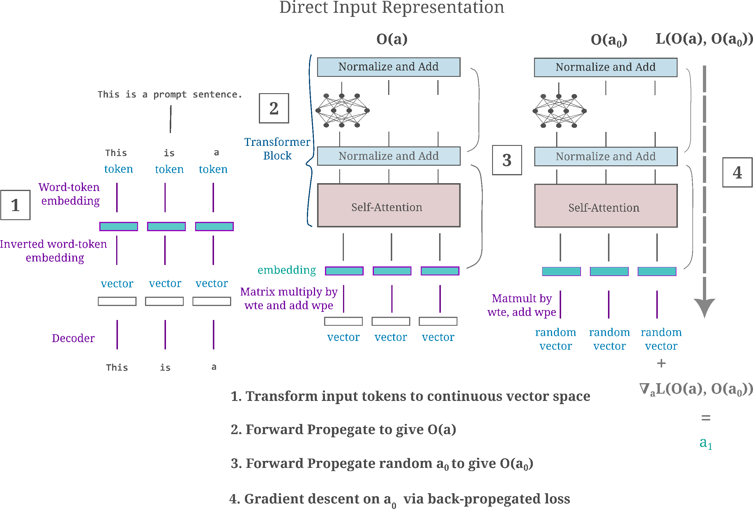
With this direct gradient descent method, can a single trained transformer block in GPT-2 be inverted accurately? Given the input
\[a = \mathtt{This \; is \; a \; prompt \; sentence}\]the answer is no: iterating \eqref{eq5} such that $\vert \vert O_l(a_g, \theta) - O_l(a, \theta) \vert \vert < \vert \vert O_l(a’, \theta) - O_l(a, \theta) \vert \vert$ (where $a’$ is a slightly shifted $a$ such that the tokenization of these vector values are identical) we have
 precarious NeighNASA Someonetre
lisherusersExp qualifying windshield
 ple propose18 joyful Genie
SHIP Geh lesbians inquiries Mat
1968 Carroll delibericycle consumers
Even when we limit the possible tokens to a very restricted set, specifically the tokens
This is a prompt sentence with some extra words attached to increase the allowed vocabulary by a small margin
and optimizing \eqref{eq5} such that the inequality denoted above is observed, we have
\[a_g = \mathtt{This \; some \; by \; small \; is}\]indicating that a single trained GPT-2 transformer block is incapable of accurate input representation even for a restricted input vocabulary, even when the input is used to perform the gradient descent. This is also true when the gradient of \eqref{eq5} is calculated using the $L_2$ norm, indicating that it is not the choice of $L_1$ norm that prevents accurate input representation here.
The same results are observed for one transformer embedding transformation and first block of the 1.5B parameter gpt2-xl model, such that neither the trained nor untrained model subsets are capable of accurate input representation even when the vocabulare is extremely limited.
For example, the top-5 decoding for the input ‘This is a prompt sentence’ for the word-to-embedding transformation followed by the first transformer block of an untrained gpt2-xl model is
 ple NeighNASA inquiries windshield
 duplusers 131 qualifyingtre
rypted Sharif deliber camping Genie
1968 Carroll maleicycle Humanity
 precariouscandExp semen consumers
and for the trained model’s embedding followed by the first transformer block, the top-5 input representations for the same prompt are
  silenced oppression Fav positioned�
 Shows debugprint interference Deploy
 softened949313 absent transports
 Ambrose mono unanswered chantingAM
ogacessive dungeonJR785
There is a clear explanation for why the GPT-2 embedding transformation is non-invertible: the linear transformation corresponding to the token-to-embedding operation transforms a vector space of dimension $d(a) = 50257$ to a vector space of $d(O_e(a, \theta)) = 728$ for the base GPT-2 model, or $d(O_e(a, \theta)) = 1600$ for the 1.5B parameter gpt2-xl. Non-invertibility is expected for both embeddings being that the output dimension is much smaller than the input, and as the input dimension exceeds the output there are many different inputs that will yield one identical output of the word to embedding transformation.
But elsewhere we have seen that non-invertible transformations can be effectively inverted using gradient descent, in the sense that an accurate input representation can be made accross non-invertible transformations. Thus it remains to be seen whether direct input representations can be accurate for other models, even if they are not accurate for GPT-2.
Multiple hidden layer outputs do not improve input representation
Why do trained language models exhibit such poor input representations? In the previous section, we found that the largest version of GPT2 exhibits far less repetition in its input representations than the smallest version of the same model. Unfortunately it is also clear that the larger model is no more capable of producing a coherent input representation (even for one transformer block) even after 1000 gradient descent iterations, corresponding to a generated distance <1/6 the magnitude of the shifted distance.
It may also be wondered whether or not input representation would be improved if we used the output of multiple layers rather than only one. For the first three layers of a model in which we perform gradient descent on the input directly, this could be implemented as follows:
class InputGPT(nn.Module):

	def __init__(self, model):
		super().__init__()
		self.model = model

	def forward(self, x: torch.tensor) -> torch.tensor:
		# replaces wte transformation
		x = torch.matmul(x, self.model.transformer.wte.weight)

		o1 = self.model.transformer.h[0](x)[0]
		o2 = self.model.transformer.h[0](o1)[0]
		o3 = self.model.transformer.h[0](o2)[0]
		output = torch.cat((o1, o2, o3))
		return output
But the input representations resulting from this are no better than before, and appears to confer the same ability to accurately represent an input as simply taking the output of the last (in this case the third) block.
Indirect input representation via cosine similarity
Another possibility is that the metric we are using to perform gradient descent is not idea for input representation. Specifically, instead of minimizing the $L^1$ metric
\[m = || O(a, \theta) - O(a_g, \theta) ||_1\]we can instead maximize the cosine similarity (ie the cosine of the angle $\phi$) between vectorized (ie flattened) versions of the output of the target input’s embedding $O(e, \theta)^* $ and the vectorized output of the generated input embedding at iteration $n$, $O(e_n, \theta)^*$
\[\cos (\phi) = \frac{O(e, \theta)^* \cdot O(e_n, \theta)^* }{||O(e, \theta)^* ||_2 * ||O(e_n, \theta)^* ||_2}\]such that gradient descent on the embedding $e_n$ is performed as follows:
\[e_{n+1} = e_n - \eta \nabla_{e_n} \left( 1 - \cos (\phi) \right)\]where $\eta$ is a tunable learning rate parameter. Performing gradient descent on the input of the first transformer block of a trained GPT-2 to minimize $\cos(\phi)$ turns out to lead to no more accurate input embeddings than before: increasing $\cos (\phi)$ to $0.96$ via 500 iterations yields embeddings that may be inverted to give
[] become Holiday trollingMa calls
 UnierierylCAP PearlOTA
Hard obviousbys abiding�士73
arcer underCoolmanship autobiography outcomes
 slog bringsquaDirgap {:
Even for a very limited vocabulary (‘The sky is blue or red depending on the time of day.’) the one transformer decoder module from GPT-2 cannot accurately represent the input, although a significant improvement is made.
\[\mathtt{This \; attached \; with \; prompt \; sentenceThis.}\]Therefore gradient descent is successful in minimizing the cosine distance between the output of the generated and target input (in this case embedding), but the generated input corresponds to nonsense. The same is true even for single transformer decoders from untrained GPT-2 models, and as we earlier found that these modules can yield accurate input representations using gradient descent on the $L^1$ norm of the output difference, the cosine similarity may be viewed as a weaker measure for representation tasks.
Perhaps a linear combination (parametrized by constants $\alpha, \beta$ of the gradient of the cosine distance and a normed difference would be sufficient for accurate input representation from trained GPT-2 transformer modules. Specifically we can see if the following update on the embedding is capable of accurate input representation. The update we make is
\[e_{n+1} = e_n - \eta * \nabla_{e_n} \left( \alpha (1 - \cos (\phi)) + \beta ||O(a_g, \theta) - O(a, \theta)||_1 \right)\]where $\eta$ is the learning rate hyperparameter, which is typically scheduled such that $\eta = 1 \to \eta = 1/100$ as the input representation iterations $n = 0 \to n = N$. But even for this metric the input representation after only one transformer encoder is quite inaccurate: for the first transformer block of an untrained GPT-2, we have input representations for ‘The sky is blue.’
 execute228 therein blue.
 politicians jihadist18having Phill
 Given patriarchal Lightning Hughes sem
� discriminatelich antitrust fraternity
ucking demos� underrated310
which means that the linear combination is less accurate than using the $L^1$ norm loss alone.
Model Interpretability
Given the extreme difficulty in accurate input representation typical of large language models when using gradient descent on an initially random input, it may be wondered whether the gradient on the input is capable of offering any useful information. This may be tested in a number of different ways, but one of the simplest is to observe what is termed input attribution. In the context of autoregressive language models trained for causal language modeling (ie predicting the next token), input attribution may be thought of as the importance of each prior token in predicting that next token.
How does one take a model and find which elements in the input are most responsible for the model output? In this case the model gives the next token in a sentence, and the input is composed of all prior tokens. We will briefly explore two options for finding the ‘most important’ input elements for a given output, although this is by no means a comprehensive survey of the field of input attribution.
One method is to find the gradient of the output with respect to each input element and multiply this gradient element-wise to the input itself. This method is known as ‘gradientxinput’ and may be found as follows:
\[v = | \nabla_a O(a, \theta) | * a\]where the vector of inputs is $a$ and the vector of saliency values is $v$ and $* $ denotes Hadamard (element-wise) multiplication, and $\vert * \vert$ signifies the element-wise absolute value operation. This method is intuitively similar to measuring the effect of an infinitesmal change in the input (via the gradient of the output $O(a, \theta)$ with respect to the input $a$) on the output, which a larger output change at index $i$ resulting in a larger saliency value at that index.
Another approach is to simply remove each input element sequentially and observe the change in the ouput. If $a_c$ correponds to the input where the token at position $c$ is replaced with an informationless substitute (perhaps a $<\vert PAD \vert >$ token) then we can find a metric distance between the model’s output given this masked input compared to the original $a$ as follows:
\[v = || O(a_c, \theta) - O(a, \theta) ||_1\]Here we use the $L^1$ metric as a measurement of the difference between outputs, but we could just as easily have chosen any other metric. This method is appropriately termed ‘occlusion’ after the English word for ‘make obscure’. This is in some ways the discrete counterpoint to saliency, as here we are observing what happens to the output after a big change (replacement of an entire token).
For small input sequences, we can form a linear combination of occlusion and gradientxinput in order to include information from both attribution methods. For longer sequences, occlusion becomes prohibitively expensive for LLMs and therefore it is usually best to stick with saliency.
To visualize input attribution on sequences of text, we can implement an HTML-based highlighter on the decoded input tokens as follows:
	def readable_interpretation(self, decoded_input, metric='combined'):
		...

		# summed_ems is a torch.tensor object of normalized input attributions per token
		positions = [i for i in range(len(summed_ems))]

		# assemble HTML file with red (high) to blue (low) attributions per token
		highlighted_text = []
		for i in range(len(positions)):
			word = decoded_input[i]
			red, green, blue = int((summed_ems[i]*255)), 110, 110
			color = '#{:02x}{:02x}{:02x}'.format(red, green, blue)
			highlighted_text.append(f'<span style="background-color: {color}">{word}</span>')

		with torch.no_grad():
			embedded_inputs = torch.clone(self.model.transformer.wte(self.input_ids))
			output = self.model(inputs_embeds=embedded_inputs)[0][:, -1, :]
			predicted_word = self.model(self.input_ids)[0][:, -1, :] # should be equal to output
			assert torch.equal(output, predicted_word)

			predicted_word = int(torch.argmax(predicted_word, dim=1))
			predicted_word = tokenizer.decode(predicted_word)

		highlighted_text = ''.join(highlighted_text)
		highlighted_text += f'</br> </br> Predicted next word: {predicted_word}'
		with open('data.html', 'wt', encoding='utf-8') as file:
			file.write(highlighted_text)
		webbrowser.open('data.html')
This function displays the relative attribution (importance) of each previous token by assigning the attribution value to the red highlighter color, while keeping green and blue highlighter values constant (see the snippet below). This makes higher-attribution tokens appear red, medium-attribution orange and grey, and low-attribution tokens green-blue.
red, green, blue = int((summed_ems[i]*255)), 110, 110
color = '#{:02x}{:02x}{:02x}'.format(red, green, blue)
After loading our model of choice, we can use this module (contained in the GPTEval class, see the source code for more information) to generate input attribution maps as follows:
if __name__ == '__main__':
	input_sequence = 'The wipers on the bus go swish swish'
	input_sequence = input_sequence.strip()
	gevaluate = GPTEval(model, input_sequence)
	input_ids = gevaluate.input_ids[0]
	decoded_input = []
	for symbol in input_ids:
		decoded_input.append(tokenizer.decode(symbol))
	arr = gevaluate.readable_interpretation(decoded_input, metric='combined')
which when given the prompt ‘The wipers on the bus go swish swish’ for the base model of GPT-2 gives
The wipers on the bus go swish swishPredicted token: sw
Observing input attribution for larger models applied to more complicated inputs, it is clear that the gradient of a model’s output with respect to its input does indeed give useful information. This being the case, we are left with the question we had at the start of this page: why are input representations so inaccurate for trained GPT-type transformers applied to natural language, and indeed why are they less accurate than for untrained models of the same type.
Sequential Input Representation
Continuing our efforts to understand why trained GPT-2 models give such poor input representations compared to trained vision transformers, one can observe that there are two notable differences between language and image inputs: language is fundamentally sequential and discreet whereas images are approximately continuous and of no particular orientation. In this section we consider the importance of the sequential aspect of language as it relates to input representation, and in the next section discreeteness is examined.
To rephrase the topic for this section, one may wonder whether or not the sequential aspect of language could contribute to difficulties in input representation. Specifically, observe that GPT-type language models always predict one word at a time, and thus may be better at representing one word at a time too.
We can implement this sequential input representation technique as follows:
def generate_sequential_input(model: torch.nn, target: torch.tensor, lr=0.5) -> torch.tensor:
	n_tokens = len(target[0])
	full_input = []
	embedding_dim = target.shape[-1]
	starting_input = torch.randn(1, 1, embedding_dim).to(device)
	combined_input = torch.clone(starting_input)
	for i in range(n_tokens):
		random_input = torch.randn(starting_input.shape).to(device)
		focused_target = target[:, i, :]
		single_input = octave(random_input, focused_target, 2000, [lr, lr/10], i) # generate single token's embedding
		combined_input = torch.cat((combined_input, single_input), dim=1)

	return combined_input[:, 1:, :]
For an untrained model given the input
\[a = \mathtt{The \; sky \; is \; blue.}\]we have a top-5 input representation of
 Pegasus quarantine Sunshine viral Dip
 secure Help Orion Saadesh
 partic Carbon Officereller Rory
 checked regained midst ERAtile
 criticize231 SOFTWARE trunkmatically
and therefore we conclude that it is not the sequential characteristic of language that is the cause of poor input representation.
Is the trained word to token embedding to blame
It might also be wondered whether the loss of input representation ability during training is due to the model learning a poorly conditioned token embedding transformation. We can test this hypothesis by replacing the trained token embedding transformation with a non-trained one, and for the direct input generation method earlier on this page this can be implemented by simply swapping the weight matrix of the word-token embedding with an untrained model’s version of the same.
class InputGPT(nn.Module):

	def __init__(self, model, untrained_model):
		super().__init__()
		self.model = model
		self.untrained_model = untrained_model

	def forward(self, x: torch.tensor) -> torch.tensor:
		# replaces wte transformation
		x = torch.matmul(x, self.untrained_model.transformer.wte.weight)

		for i in range(1):
			x = self.model.transformer.h[i](x)[0]
		return x
However, we are not met with any success in making even one transformer block yield accurate input representations.
 veiledusers lesbians inquiries windshield
 dupl NeighNASAicycletre
rypted IntExp qualifying Genie
 melts funded deliber camping Mat
SHIP rejoice malepc consumers
Similarly poor input representations are exhibited when we use the Roy-Moore pseudo-inverse indirect input generation method following the
PsyNetMessagePsyNetMessagePsyNetMessage MarketablePsyNetMessage
 srfAttach srfAttach MarketablePsyNetMessage srfAttach
irtual unfocusedRange unfocusedRange unfocusedRange partName
 partName Marketable srfAttachawaru Marketable
ascus partName partName srfAttach unfocusedRange
In conclusion, we find that the training of the embedding transformation alone cannot account for the poor representation that exists in trained language models. This does not necessarily mean that the embedding transformation does not affect input representation, but only that the process of training the embedding alone does not account for the poor input representation in GPT-2 models after training.
Big models exhibit accurate input representations
It has been claimed that language models as they exist today are incapable of any kind of fact- or reason- based task because they are merely trained to predict the next word (or more accurately token) in some text. We can show that this claim is incorrect, however, using a fairly straightforward argument. We can define a language model as some generalizable (to examples unseen in the training data) representation function that maps input token sequences to an output token such that the negative log-likelihood of that output token is minimized relative to the training dataset.
From this definition alone we find that language models must also be capable of all the implicit tasks present in the training dataset. For example, suppose the training data contained the phrase ‘two plus two equals four’. Given the input ‘two plus two equals’ the function must return ‘four’ if it has minimized the negative log-likelihood of that token. Now suppose the training data also contains the phrase ‘four plus one equals five’ and that now we give the unseen phrase ‘two plus two plus one equals’ and our function returns a token. If our function is sufficiently generalizable, we are almost guaranteed to return ‘five’ because the internal representation of ‘two plus two’ is nearly equivalent to ‘four’ and the model has already learned that ‘four plus one equals five’.
It has been empirically observed that models with more parameters are generally better at these implicit natural language tasks, which typically lie under the umbrella definition of ‘reasoning’ problems. There are a few explanations for why this could be: firstly, larger models entail higher-dimensional space, such that gradient descent is more biased towards generalization, secondly because more parameters imply greater ‘memory’ such that the model can learn more complicated representations of an input (ie ‘three’ being both a word and an implicit number) and thirdly because it is apparent that biological neural networks require a very large number of neurons to deal with language relative to other tasks, such as object recognition.
But when we have observed that although larger models (~1 billion as opposed to 100 million parameters) tend to have less repetition, they are no noticeably better at input representation than smaller models (~100M parameters). Do even larger models fail to exhibit accurate input representation? We can investigate by observing the ability of our gradient descent procedure to autoencode an input from transformer models of a trained GPT-J model, which contains ~6B parameters. To save memory, we can load the parameters in 8-bit format using bitsandbytes
load_8bit = True
tokenizer = AutoTokenizer.from_pretrained("EleutherAI/gpt-j-6b")
model = AutoModelForCausalLM.from_pretrained("EleutherAI/gpt-j-6b", load_in_8bit=load_8bit, device_map='auto')
GPT-J, like Llama and other transformer models used today, employs Rotary Positional Encoding that is applied to each attention module (introduced by Su and colleagues). This means that there is no wpe transformation to invert, but we instead have to supply the appropriate positional information as position_ids to each transformer block. Using the indirect input generation method in which gradient descent is performed on the first hidden layer before the resulting tensor is inverted, the modifed version of a trained GPT-J model may be specified as follows
class AbbreviatedGPT(nn.Module):

    def __init__(self, model):
        super().__init__()
        self.model = model

    def forward(self, x: torch.Tensor):
        position_ids = torch.tensor([i for i in range(x.shape[1])])

        for i in range(1):
            x = self.model.transformer.h[i](x, position_ids=position_ids)[0]
        return x
Here we investigate the representations present various layers of a model using gradient descent on the embedding of a discrete language input, a technique explained here. For the prompt ‘The sky is blue.’ after $N=200$ iterations with the first transformer block of GPT-J, we generate an $a_g$ such that $\vert \vert a_g - a \vert \vert < \vert \vert a’ - a \vert \vert$ which yields the top-5 token matching of
The skyeton resp cease
hinPresidentVER compose Instruments
uddinuko be blue_
JJzbuse Oxy rite
earlyerent iswn seasoning
which is certainly somewhat better than we saw for the smaller models. Note, however, that even at $N=2000$ the input representation accuracy is not sufficient to unambiguously identify the input string.
On the other hand, if we restrict the input tokens to any of ‘The sky is blue or red depending on the time of day.’ we come very close to recovering the input.
\[a_g = \mathtt{The \; sky \; is \; blue \; of}\]Which is a notable improvement upon the smaller trained models seen previously.
This begs the question: would an even larger model be capable of even more precise input representation? We can check this using various models but one in particular is the Llama model family introduced by Touvron and colleagues, which may be loaded in 8-bit parameter quantization as follows:
tokenizer = AutoTokenizer.from_pretrained("huggyllama/llama-13b")
model = AutoModelForCausalLM.from_pretrained("huggyllama/llama-13b", load_in_8bit=load_8bit, device_map='auto')
Llama models name their components somewhat differently than GPT-type models, and apply Rotary Positional Encoding via different dimensions, so after consulting the source code we subclass the model as follows:
class AbbreviatedGPT(nn.Module):

    def __init__(self, model):
        super().__init__()
        self.model = model

    def forward(self, x: torch.Tensor):
        position_ids = torch.tensor([[i for i in range(x.shape[1])]])

        for i in range(4):
            x = self.model.model.layers[i](x, position_ids=position_ids)[0]
        return x
This model requires around 20GB when performing the gradient descent input representation algorithm, so the following experiments are performed using an Nvidia A100 GPU (available on Colab for a fee).
After $N=1000$ we have for the first transformer block:
\[a_g = \mathtt{the \; sky \; the \; blue \; }\]and at $N=2000$ we have the top-5 representations of
The sky is blue’
K Sky isn Bluerows
’sky’Blue K
The K Kativecards
rowsXrows K?"
and even more remarkably, at a depth of two transformer blocks for $N=2000$ the model’s representation is
\[a_g = \mathtt{The \; sky \; is \; blue.}\]which means that we have found a way to get accurate input representations from a trained transfomer block! Apparently the we simply have to use an extremely large model. Thus we would expect to observe accurate input representations from even larger models, and we test this using the 30 billion parameter version of Llama (which is about the largest model that will fit in the memory of a 40GB A100 using 8-bit quantization). For the first transformer block of this trained model after a mere $N=500$ we have top-5 representations of
The sky is blue<s>
� Sky: Blue “
Helpsky�Blueww
smart Japan behblueATCH
cy Answer� explating
where <s> signifies a sentence break token (which is nearly identical with a period in semantic meaning).
Compare this with the top-5 representations of the first transformer block of a 7-billion parameter version of Llama, which at $N=500$ gives
The sky isYS2
The ofATIONhere-
..�althOIN

,SE ${\reno
the
c blue,
although it should be noted that if the maximum number of gradient descent iterations $N$ increases to $N=1500$, the 7b parameter Llama yields a better
\[a_g = \mathtt{The \; sky \; is \; blue2}\]With the 30 billion parameter Llama, we find that at least somewhat accurate input representations are made from deeper and deeper layers: representation after 4 transformer blocks is qualitatively similar to what is found for 1 block (above) even after 12 (!) transformer blocks, we get a recognizable input representation of
\[a_g = \mathtt{The \; sky \; Stage \; blueInd}\]Note that with the 7 billion parameter version of Llama, a typical top-5 representation of the input at a depth of 12 blocks for the same $N$ is
havior skyichtetfiterson
burgје speakeriffsbled
prisoners prisoners standardsunct speaker
learn studying relationshipsspanburg
rium Cup containingEEali
meaning that we find much poorer input representations in the 7b parameter Llama as opposed to the 30b model in the deeper layers, which is to be expected with the hypothesis that larger models are capable of transmitting input information more accurately than small ones.
Returning to the 30 billion parameter model, even after 21 transformer blocks the input representation is nearly synonymous with the prompt.
\[a_g = \mathtt{Finally \; sky \; established \; blue \; instead}\]This is notable because smaller language models are capable of accurate input representation before training, but only for one or at most two transformer blocks. But with increased model size, trained models are capable of fairly accurate input representation even in relatively deep layers.
It may also be wondered whether we can recover accurate input representations by optimizing a different metric on a hidden layer output. Earlier on this page we saw that cosine similarity used as a metric for GPT-2 models was incapable of accurate input representation, but it is worth exploring whether this is the case now that we have a larger model to work with. As before, we perform gradient descent on the embedding $e_n$ rather than a vectorized input.
A first experiment is not promising: given the same prompt as above (‘The sky is blue’) after $N=500$ iterations of gradient descent on the embedding of an input such that $\phi < 0.05$ we have
\[a_g = \mathtt{WNWNWNWN}\]but the slight change to ‘The sky is blue.’ yields
\[a_g = \mathtt{The \; sky \; is \; blue2}\]Longer prompts such as ‘The sky is red or blue depending on the time of day’
\[a_g = \mathtt{The \; sky \; is \; blue \; or \; red \; depending \; on \; the \; time \; OF \; day}\]or ‘This is a prompt sentence.’
\[a = \mathtt{This \; is \; a \; prompt \; sentence.}\]We find the same tendancy for poorer input representations at deeper layers (observed above for an L1 metric distance loss) to be the case for cosine similarity loss too. For example, at block 4 of Llama 7b we have
\[a_g = \mathtt{This \; is \; a \; prompt \; sentence \; SU}\]but at block 12 we have
\[a_g = \mathtt{Thusieraución \; prompt \; Jersey \; Culture}\]Large models exhibit poor direct input representation when minimizing hidden layer L1 distance but not cosine similarity
In the last section we saw that very large models are capable of accurate indirect input representation when gradient descent performed on the input embedding, rather than directly on the input itself. It may be wondered whether similarly accurate input representations are found from the same models if gradient descent is performed on the inputs diectly, after converting discrete token integers to a continuous vector space equivalent to those discrete tokens.
For Llama-type models that use RoPE, after converting a tokenized input into a vector-space equivalen x we can sub-class our chosen model as follows:
class InputModel(nn.Module):

	def __init__(self, model):
		super().__init__()
		self.model = model

	def forward(self, x: torch.Tensor):
		# Matrix mult instead of embedding to prevent type incompatibility
		x = torch.matmul(x, self.model.model.embed_tokens.weight)
		position_ids = torch.tensor([[i for i in range(x.shape[1])]])

		for i in range(1):
			x = self.model.model.layers[i](x, position_ids=position_ids)[0]
		return x
Given the target input $a = \mathtt{This \; is \; a \; prompt \; sentence}$, the trained 7 billion parameter Llama model yields the following top-5 input representations at the output of the first transformer block:
sout spectconmicadém
Normdatei┴więひ
Son画 hastaрук cb
ccCollectennenzen Kirchen
alusEmemed expon.<
We find further that the trained 30 billion parameter Llama model is similarly incapable of accurate direct input representation. For $N$ such that $\vert \vert O(a, \theta) - O(a_g, \theta) \vert \vert < \vert \vert O(a, \theta) - O(a’, \theta) \vert \vert$ we have
льной розта Schw университета ded
nombreuses мат FemAvailable modify
Cés projection polygonダjekt
`" помо э dll физи
dai vba грудняóp поль
It may be wondered whether or not a different metric would give a more accurate input representation, at least for the first transformer block of Llama 7b.
To be more precise, we want to minimize the angle $\phi$ between the vector corresponding to the hidden layer output of some target input $a$ and a generated input $a_g$ by maximizing the cosine similarity between the output of the target input $a$, denoted $O(a, \theta)$ and the generated input $a_g$, $O(a_g, \theta)$ via gradient descent on an initially random input $a_0$. The cosine distance may be calculated on vectorized versions of these outputs, denoted $O()^*$, as follows:
\[\cos (\phi) = \frac{O(a, \theta)^* \cdot O(a_g, \theta)^* }{||O(a, \theta)^* ||_2 * ||O(a_g, \theta)^* ||_2}\]such that gradient descent on a vectorized version of the input $a_n$ as follows:
\[a_{n+1} = a_n - \eta \nabla_{a_n} \left( 1 - \cos (\phi) \right)\]Maximizing the cosine similarity (ie minimizing the angle $\phi$) between generated input $a_g$ and target input $a$ yields for the $a$ given above
\[a_g = \mathtt{This \; is \; hasta \; prompt \; sentence}\]where $(\cos(\phi) > 0.9$.
For
\[a= \mathtt{This \; is \; a \; somewhat \; longer \; prompt \; sentence.}\]we have at $\cos(\phi) = 0.76$
\[a_g = \mathtt{This \; are \; integrated \; somewhat \; longer \; prompt \; sentence –}\]For another target sentence
\[a = \mathtt{The \; sky \; is \; a \; light \; blue \; today.}\]at $\cos(\phi=0.75)$ we have
\[a_g = \mathtt{primit \; sky \; is \; a \; light \; blue \; today \; –}\]It is interesting to note that cosine similarity loss does not yield accurate input representations for small inputs. For example, given $a = \mathtt{The \; sky \; is}$ the first block representation is
\[a_g = \mathtt{sier \; fixeseden}\]Nearly every one-word target input gives very inaccurate input representations, with $a_g$ as any of ‘George’, ‘The’, ‘when’, or ‘clearly’ yielding $a_g = \mathtt{que}$, and inputs with two or only a few words are often quite inaccurately representation via cosine similarity.
prompt = 'Boba Fett'
Nacional**** têteстори

prompt = 'Boba Fett was a bounty hunder'
фами函WNזWN поддерpersoninasacjęлище

prompt = 'Boba Fett was a legendary bounty hunter in the outer rim'
Boba Fett wasondissement legendary bounty hunter in the outer rim
This is a marked contrast from performing gradient descent on the input embedding, where cosine similarity yields accurate representations even for one-word inputs (ie ‘George’ is represented ‘George’).
Why would the use of cosine similarity be unable to give accurate input representations when applied to input space of very small inputs but not larger ones? It is helpful to consider here what exactly is being optimized: the cosine of $\phi$ is equal to the dot product of two vectors divided by the norms of those vectors multiplied together.
Cosine loss optimization and model training
Why is direct input representation so inaccurate for single token inputs, even though it is accurate for multi-token inputs? Consider that the self-attention module in the Llama transformer blocks are based on the dot product operation: the attention between any query $q$ token and a key $k$ token is given as
\[A(q, k, v) = \mathrm{softmax} \left( \frac{q \cdot k}{\sqrt(d)} \right) v\]Recalling that the dot product is equivalent to the cosine of the angle between vectors $q, k$ divided by their norms, one can say that attention compares the direction between these vectors.
But something unexpected occurs when we attempt to use cosine similarity as a metric for an untrained Llama model: for one-token inputs gradient descent is able to minimize $\cos (\phi)$ on the output of any given transformer block, but when more that one token is present in the input this is no longer possible.
We can deconstruct the transformer block by investigating the LlamaDecoderLayer module from the Llama source code and replicating that module in pieces as follows.
class InputGPT(nn.Module):

	def __init__(self, model):
		super().__init__()
		self.model = model

	def forward(self, x: torch.Tensor):
		# Matrix mult instead of embedding to prevent type incompatibility
		x = torch.matmul(x, self.model.embed_tokens.weight)
		position_ids = torch.tensor([[i for i in range(x.shape[1])]])

		for i in range(1):
			residual = x
			x = self.model.layers[i].input_layernorm(x)
			x = self.model.layers[i].self_attn(x, position_ids=position_ids)[0] + residual
			residual = x
			x = self.model.layers[i].post_attention_layernorm(x)
			x = self.model.layers[i].mlp(x) + residual

		return x
It turns out that removing the layer normalizations allows minimization of $\cos (\phi)$ on the output via gradient descent on the input, as long as the input is not too long (>5 tokens). This is suggestive of a numerical underflow or overflow in the gradient backpropegation process, which appears to be exacerbated by the layer normalization transformations.
Back to the question of whether untrained Llama models are capable of accurate input representation, we find that it is both more difficult to minimize $\cos(\phi)$ via gradient descent and that once minimized, the inputs are not accurate the the target $a$. For $\cos (\phi) < 0.15$ we have
\[a = \mathtt{The \; sky \; is \; blue} \\ a_g = \mathtt{ПерViewModeldfrac \; paths}\]It should be noted that untrained models appear to be worse at indirect input representation as well, as for the prompt $a = \mathtt{The \; sky \; is \; blue}$ the first transformer block from an untrained 7b Llama gives
\[a_g = \mathtt{leaf \; leaf \; Connect \; leaf}\]at $N=1500$, whereas the trained model is much more accurate (see above).
But upon some reflection, it may not be surprising that minimizing a cosine distance between outputs of an untrained transformer block does not yield accurate input representations because the dot-product attention is followed by two fully connected layers. If we instead observe the representation from the first ransformer block’s self-attention whilst minimizing $\cos \phi$,
class InputGPT(nn.Module):

	def __init__(self, model):
		super().__init__()
		self.model = model

	def forward(self, x: torch.Tensor):
		position_ids = torch.tensor([[i for i in range(x.shape[1])]])

		for i in range(1):
			x = self.model.layers[i].self_attn(x, position_ids=position_ids)[0]
		return x
we have a permutation of the input ‘The sky is blue.’
\[a_g = \mathtt{blue \; is \; The \; sky}\]with a top-5 representation
blue is The sky
The The sky is
sky blue is The
is sky blue blue
FLITEite период
and likewise for ‘This is a prompt sentence’ we have
\[a_g = \mathtt{prompt. \; This. \; is \; prompt}\]Although with 4 self-attention blocks, more information is lost:
\[a_g = \mathtt{sentence. \; Thisอ \; OK \; sentence}\]On the other hand, minimization of $L^1$ distance on the output of the first (untrained) full transformer block containing self-attention followed by an MLP gives
The ense The blue
sky is blue essere
pandas sky sky tör
blue land proud{$
.-- skill iseli
but for inputs composed of individual words (more precisely tokens) the representation is nearly perfect, for example any of the inputs ‘This’, ‘is’, ‘a’, ‘prompt’,’sentence’ give a representation identical to that input. As soon as the input contains multiple tokens, however, minimizing the $L^1$ distance on the output is not longer sufficient for perfectly accurate representation, for example ‘the sky’ is represented as ‘sky sky’.
Noise on a Discreet Channel
To recap, we have found that accurate input representations of images but not language are not formed in trained transformer models unless they contain a very large number of parameters.
But first it remains to be seen why training would result in worse input representations, why larger models would be capable of much more accurate representation, and above all why accurate input representation appears to be so much more difficult for language than for images.
In developing the theory of communication over a noisy channel, Shannon and others found a mathematical explanation for a phenomenon that initially seemed most curious: the fact that the amount of information reaching the receiver often decreases imperceptably at first and then suddenly plummets as the amount of information passed during a given amount of time increases, given constant noise in the channel.
It may be wonderd if the same observation would be made for deep learning models, which may be thought of as being somewhat analagous to noisy channels over which information from the input passes to the output. Indeed it is found that language model input representation experiences a severe drop as the channel width decreases. For the 7 billion parameter trained Llama with 4096 feature neurons per layer, reducing this number to 2202 yields all correct input tokens for the input ‘Mario the man versus Mario the idea’ but decreasing this by even one neuron (ie taking [:, :, :2201] in shape [batch, token, embedding] as the output used to perform gradient descent-based input optimization) leads to zero tokens being correctly represented. The same is true when we consider only the attention layers in modules (no MLPs), where the number of necesary neurons now is 2084. These observations are not due to the identity of the specific tokens being chosen, but can be thought of as a true bandwidth phenomenon: in the case of the attention-only module taking [:, :, 1000:3083] yields no token accurately found but taking [:, :, 1000:3084] gives every input token accurately, just as using the information from the first 2084 tokens yields an exactly accurate representation of the input whereas using the first 2083 tokens ([:, :, :2083]) yields a representation that cannot identify a single input token exactly.