Language Model Representations and Features

Introduction to Language

One of the most important theorems of machine learning was introduced by Wolpert and is colloquially known as the ‘No Free Lunch’ theorem, which may be stated as the following: no particular machine learning method is better or worse than any other when applied to the problem of modeling all possible statistical distributions. A similar theorem was shown for the problem of optimization (which covers the processes by which most machine learning algorithms learn) by Wolpert and Macready, and states that no one algorithm is better or worse than any other across all classes of optimization problems.

These theorems are often used to explain overfitting, in which a model may explain training data arbitrarily well but explains other similar data (usually called validation data) poorly. But it should be noted that most accurately these theorems do not apply to the typical case in which a finite distribution is being modeled, an d therefore are not applicable to cases of empirical overfitting. But they do convey the useful idea that each machine learning model and optimization procedure is usueful for only some proper subset of all possible statistical distributions that could exist.

The assumption that not all possible distributions may be modeled by a given learning procedure does not affect the performance of machine learning, if one assumes what is termed the manifold hypothesis. This hypothesis posits that the set of all elements for a given learning task (ie natural images for a vision model or English sentences for a language model) is a small subset of the set of all elements that could exist in the given space (ie all possible images of a certain resolution or all possible permutations of words and spaces). The task of the learning program is simply to find the manifold, which is the smooth and approximately connected lower-dimensional space that exists in the higher-dimensional input, such that the objective function associated with the learning task is minimized.

It has been observed on this page that subsequent layers of vision models tend to map arbitrary inputs to manifolds learned during training, rather than simply selecting for certain pieces of input information that may be important for the task at hand. The important difference is that we can see that vision models tend to ‘infer’ rather than simply select information about their input during the manifold mapping process. Typically the deeper the layer of the vision model, the more input information is lost in the untrained model and the more information that is inferred in the trained one.

We may wonder whether this is also the case for language models: to these also tend to infer information about their input? Are deeper layers of language models less capable of accurately reconstructing the input, as is the case for vision models? Do deeper layers infer more input information after training?

Spatial Learning in Language Model Features

The most prominent deep learning model architecture used to model language is the Transformer, which combines dot product self-attention with feedforward layers applied identically to all elements in an input to yield an output. Self-attention layers originally were applied to recurrent neural networks in order to prevent the loss of information in earlier words in a sentence, a problem quite different to the ones typically faced by vision models.

Thus convolutional vision and language models diverged until it was observed that the transformer architecture (with some small modifications) was also effective in the task of image recognition. Somewhat surprisingly, elsewhere we have seen that transformers designed for vision tasks tend to learn in a somewhat analagous fashion to convolutional models: each neuron in the attention module’s MLP output acts similarly to a convolutional kernal, in that the activation of this neuron yields similar feature maps to the activation of all elements in one convolutional filter.

It may be wondered whether transformers designed for language tasks behave similarly. A first step to answering this question is to observe which elements of an input most activate a given set of neurons in some layer of our language model. One way to test this is by swapping the transformer stack in the vision transformer with the stack of a trained language model of identical dimension, and then generating an input (starting from noise) using gradient descent on that input to maximize the output of some element. For more detail on this procedure, see this page.

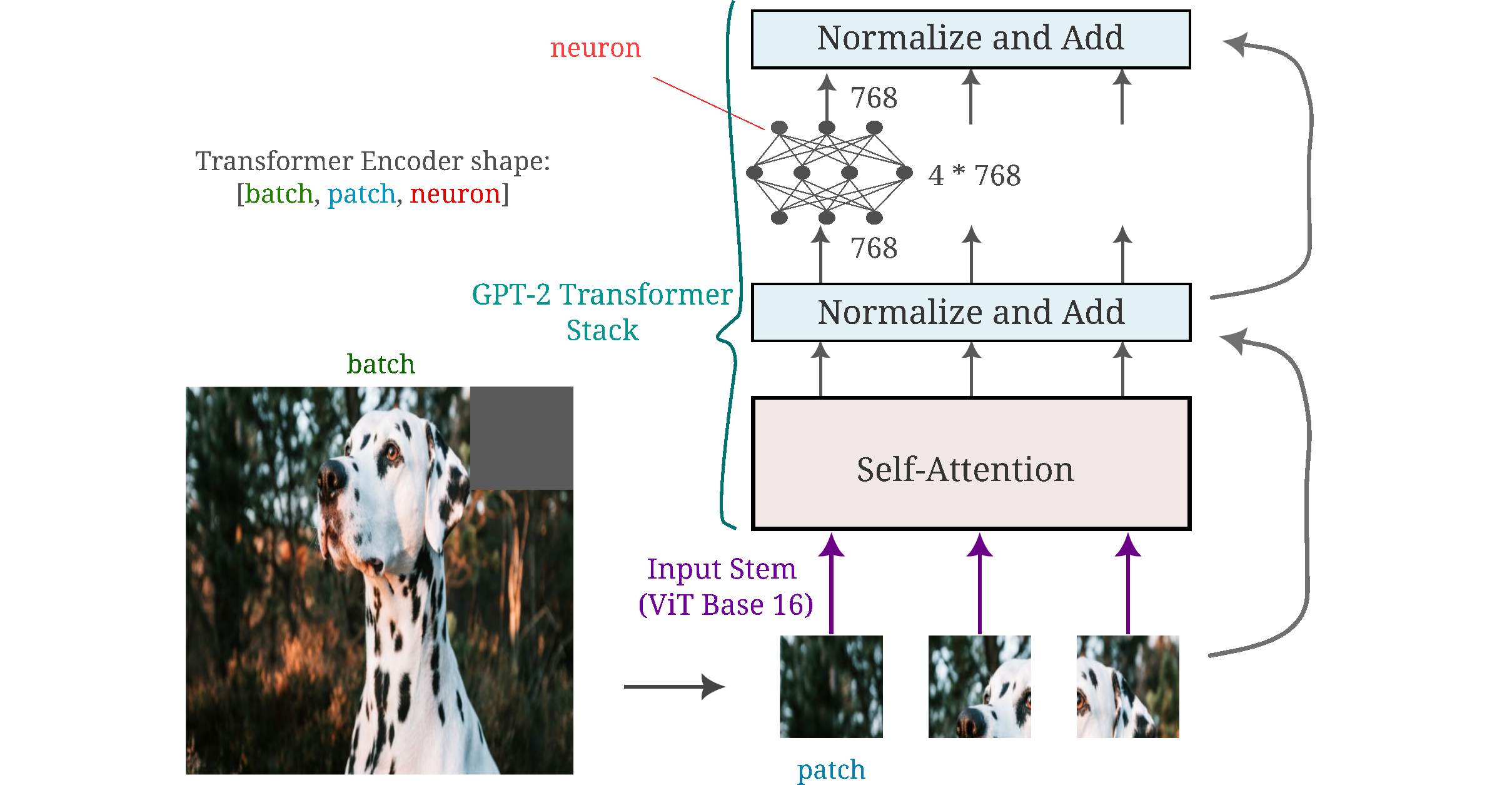
To orient ourselves to this model, the following figure is supplied to show how the input is split into patches (which are identical to the tokens use to embed words or bytepairs in language models) via the convolutional stem of Vision Transformer Base 16 to the GPT-2 transformer stack. GPT-2 is often thought of as a transformer decoder-only architecture, but aside from a few additions such as attention masks the architecture is actually identical to the original transformer encoder and therefore is compatible with the ViT input stem.

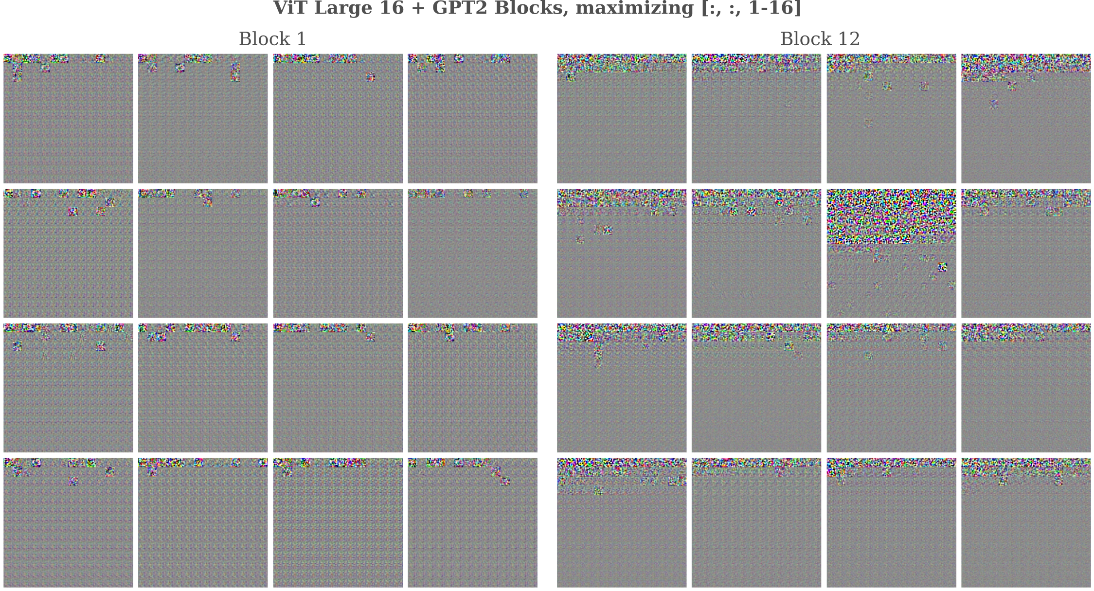
Here we are starting with pure noise and seek to maximize the activation of a set of neurons in some transformer module using gradient descent between the neurons’ value and some large constant tensor. To be consistent with the procedure used for vision transformers, we also apply Gaussian convolution (blurring) and positional jitter to the input at each gradient descent step (see this link for more details). First we observe the input resulting from maximizing the activation of an individual neuron (one for each panel, indexed 1 through 16) across all patches. In the context of vision transformers, the activation of each single neuron in all patches (tokens) forms a consistent pattern across the input (especially in the early layers).

When the activation of a single neuron in all tokens of GPT-2 is maximized using the ViT input convolution with the added transformations of blurring and positional jitter, we have the following:

The first thing to note is that we see patterns of color forming in a left-to-right and top-to-bottom fashion for all layers. This is not particularly surprising, given that the GPT-2 language model has been trained to model tokens that are sequential rather than 2-dimensional as for ViTs, and the sequence of tokens for these images is left to right, top to bottom.

It is somewhat surprising, however, that much of the input (particularly for early layers) is unchanged after optimization, implying that as the patch number increases there is a smaller chance that activation of a neuron from that patch actually requires changing the input that corresponds to that patch, rather than modifying earlier patches in the input. It is not altogether surprising that maximizing the activation of all GPT-2 tokens should lead to larger changes to the first compared to the last tokens. This is because each token only attends to itself and earlier tokens.

For an illustration of why we would expect for early input tokens to have more importance than later ones assuming equal importance placed on all inputs, consider the simple case in which there are three tokens output $t_1, t_2, t_3$ and $f’(t_n)$ maximizes the output of all input tokens $i_0, i_1, i_2$ with index $m \leq n$ equally with unit magnitude. Arranging input tokens in an array as $[i_0, i_1, i_2]$ for clarity,

\[f'(t_1) = [1, 0, 0] \\ f'(t_1, t_2) = [2, 1, 0] \\ f'(t_1, t_2, t_3) = [3, 2, 1] \\\]

In the images above we are observing the inputs corresponding to $f’(t_1, t_2, …, t_n)$. From the figure above it appears that there is a nonlinear decrease in the input token weight as the token index increases, indicating that there is not in general an equal importance placed on different tokens.

There also exists a change in relative importance per starting versus ending token in deeper layers, such that early layer neurons tend to focus on early elements in the input (which could be the first few words in a sentence) whereas the deeper layer neurons focus more broadly.

Positional jitter and Gaussian blurring convolutions are performed on vision models to enforce statistical properties of natural images on the input being generated, namely translation invariance and smoothness. There is no reason to think that language would have the same properties, and indeed we know that in general language is not translation invariant.

We therefore have motivation to see if the same tendancy to modify the start of the input more than successive layers (as well as more broad pattern of generation with deeper layers) also holds when jitter and blurring are not performed. As can be seen in the figure below, we see that indeed both observations hold, and that the higher relative importance of starting compared to ending input patches is even more pronounced.

When we instead activate all elements (neurons) from a single patch, we see that in contrast to what is found for vision transformers, early and late layers both focus not only on the self-patch but also preceding ones too. Only preceding patches are modified because GPT-2 is trained using attention masks to prevent a token peering ahead in the sequence of words. Note too that once again the deeper layer elements focus more broadly than shallower layer elements as observed above.

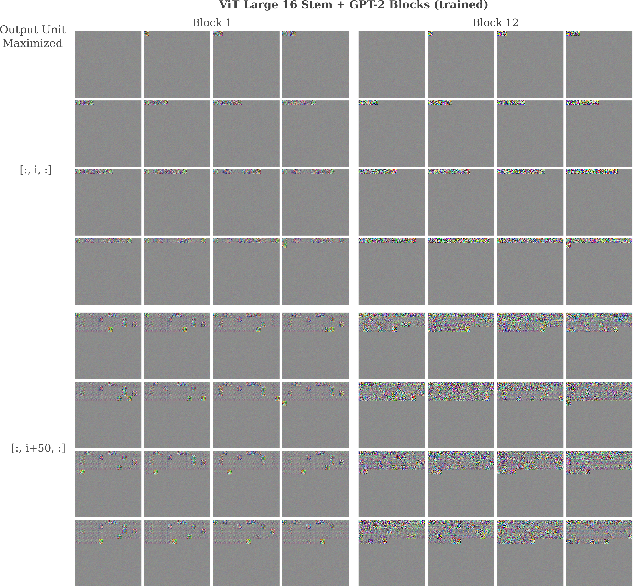
The incorperation of more global information in deeper layers is also observed for vision models, although it is interesting to note that transformer-based vision model patches typically do not incorperate as much global information in their deeper layers as MLP-based mixers or convolutional models.

Image Reconstruction with Language Models

How much information is contained in each layer of a language model? One way to get an answer to this question is to attempt to re-create an input, using only the vector corresponding to the layer in question. Given some input $a$, the output of a model $\theta$ at layer $l$ is denoted $y = O_l(a, \theta)$. Does $O_l(a, \theta)$ contain the information necessary to re-create $a$? If we were able to invert the forward transformation $O_l$, then it would be simple to recover $a$ by

\[a = O_l^{-1}(y, \theta)\]

But typically this is not possible, as for example if multiple inputs $a_1, a_2, …, a_n$ exist such that

\[O_l(a_1, \theta) = O_l(a_2, \theta) = \cdots = O_l(a_n, \theta)\]

which is the case for transformations present in many models used for language and vision modeling. Besides true non-invertibility, linear transformations with eigenvectors of very different magnitudes are often difficult to invert practically even if they are actually invertible. This is termed approximate non-invertibility, and has been seen to exist for vision models here.

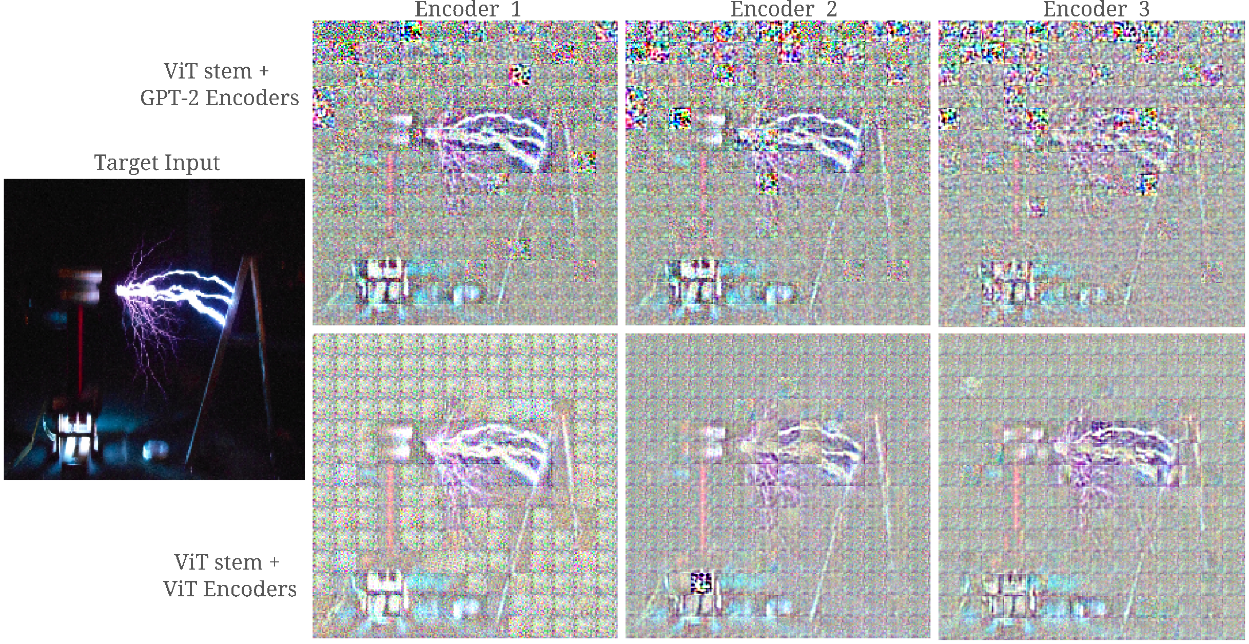
The ability of the information present in $O_l$ to generate $a$ from noise can be thought of as a measure of representational accuracy. How does representational accuracy for transformers trained for language modeling compare to those trained for image classification? In the following figure, we can see that the trained GPT-2 has less accurate input representations in the early layers than ViT Large does, although these layers are still capable of retaining enough information to generate recognizable images.

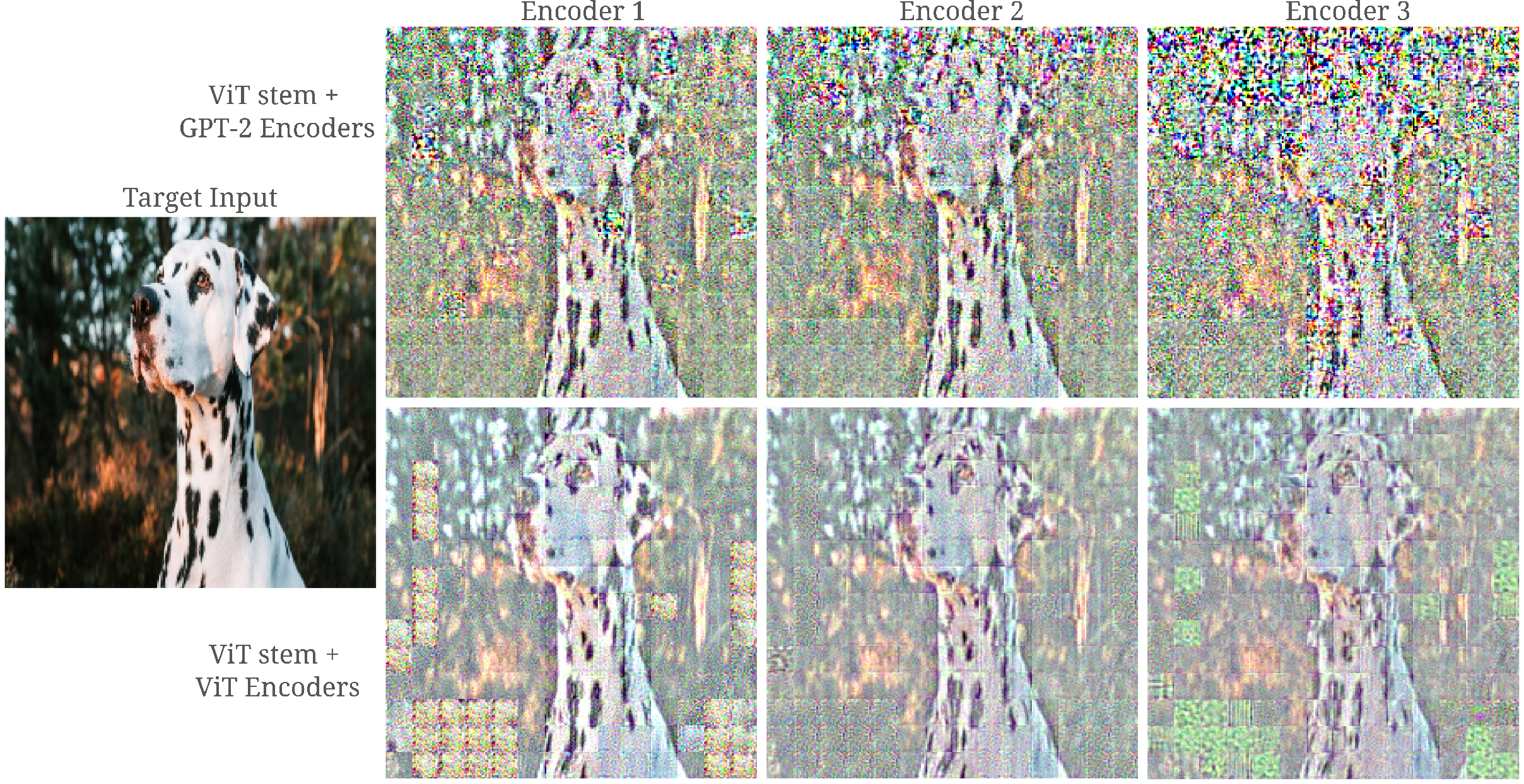
This is also the case for out-of-distribution images such as this Tesla coil. In particular, the first few dozen tokens (top few rows in the grid of the input image, that is) of the input for both images are comparatively poorly represented, and display high-frequency inputs that is common for representations of poorly conditioned models.

Conclusion

On this page we have seen that deeper modules focus more broadly on input tokens whereas shallower layers tend to focus on specific portions (here early parts) of the input. Compared with vision transformers, it is apparent that language transformers are less self-attentive such that each patch (token) tends to focus on more than itself.

In some respects, it is surprising that models designed for language processing would be capable of retaining most input information even across a single transformer block.