Sentence Representation with Language Models
In the previous section we have seen that a trained language model is less capable of representing a visual input than a trained language model (both with similar transformer architectures). Given the nature of the inputs each model type is trained on, this may not seem very unexpected. It is more informative to consider the ability of language model layer outputs to represent language inputs, rather than images. More accurate representation implies more input information passing through the model to the chosen layer’s output.
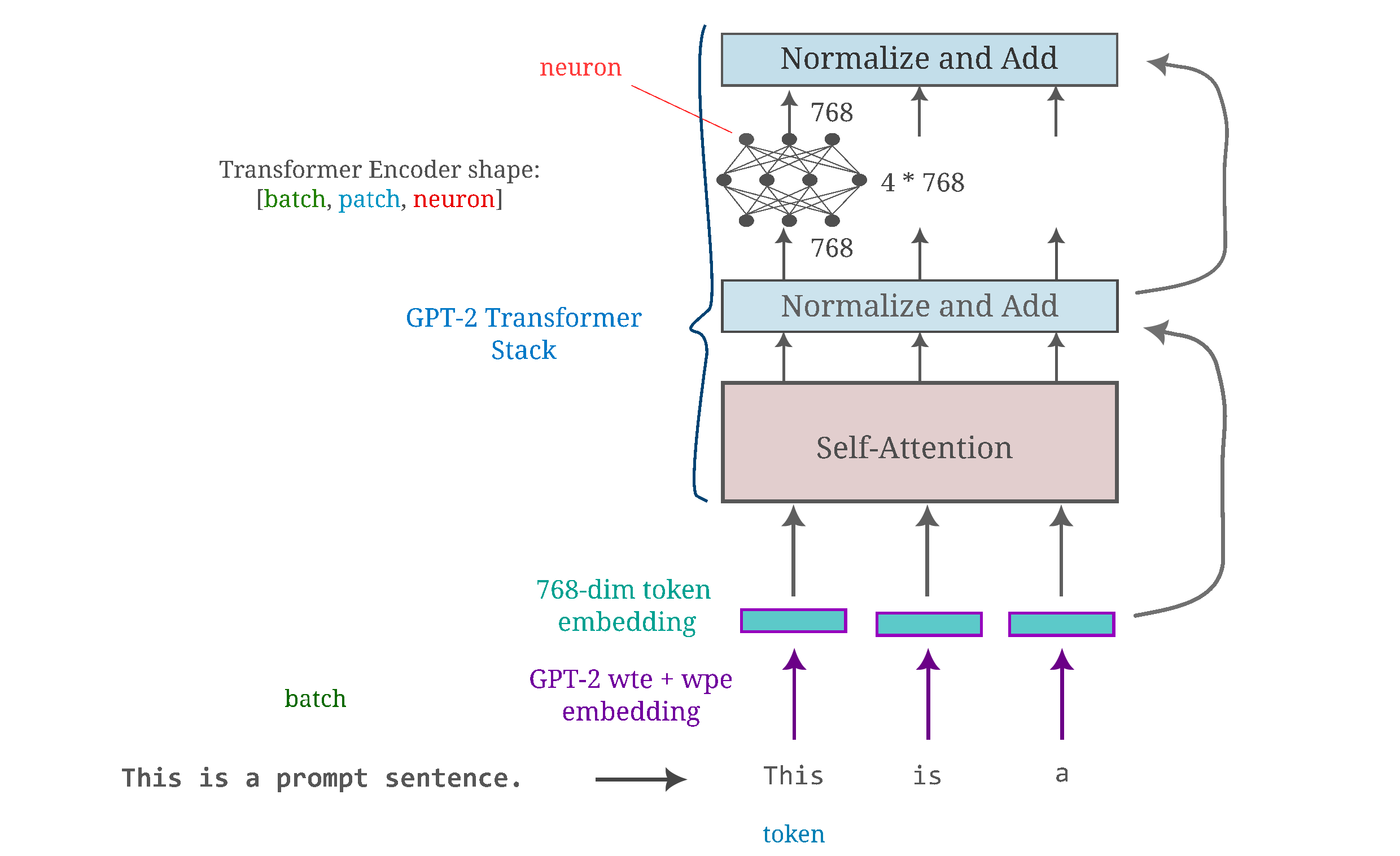
To orient ourselves, first consider the architecture of a typical transformer-based language model.
Language input generation presents a unique challenge to gradient-based optimization methods because language inputs are fundamentally discrete: a word either exists in a certain part of a sentence or it does not. This is a notable contrast to images of the natural world, where each element (ie pixel) may take any value between 0 and the maximum possible intensity of that image (which is 255. for 8-bit images) and therefore are much better approximated by continuous values.
The standard approach to observing the input information present for some vision model layer is to start with a random normal input $a_0 = \mathcal{N}(a, \mu=1/2, \sigma=1/20)$ and then perform gradient descent on some metric (here $L^1$) distance between the target output $O_l(a, \theta)$ for $N$ total iterations, each step being
\[a_{n+1} = a_n - \eta * \nabla_{a_n} ||O_l(a_n, \theta) - O_l(a, \theta)||_1 \\ \tag{1}\label{eq1}\]with $\eta$ decreasing linearly from $\eta$ to $\eta / 10$ as $n \to N$ which empirically results in the fastest optimization. The more information of the input that is retained at that layer, the smaller the value of $\vert \vert a_N - a \vert \vert$.
This gradient descent method is not useful for language models without some modifications, given that $\nabla_{a_n}$ is undefined for discrete inputs which for language models are typically integer tokens. Instead we must perform gradient descent on some continuous quantity and then convert to and from tokens.
There are two ways that we can perform gradient descent on tokenized inputs: the first is to first convert the tokens to a lower-dimensional (and continuous) embedding and then perform gradient descent on that embedding, and the other is to convert to the tokens into a $d$-dimensional vector space and modify the model to perform gradient descent such that this vector space is the input (thus the leaf node of the gradient backpropegation computational graph). We will take the first strategy for this section and only later revisit the second.
For large language models such as GPT-2, the process of conversion between a discrete token and a continuous embedding occurs using a word-token embedding, which is programmed as a fully connected layer without biases but is equivalent to a (usually full-rank) matrix multiplication of the input token vector $x$ and the embedding weight matrix $W$ to obtain the embedding vector $e$.
\[e = Wa\]As $e$ is continuous, we can perform gradient descent on this vector such that $e_g$ may be generated from an initially random input $e_0 = \mathcal{N}(e, \mu=1/2, \sigma=1/20)$.
But we then need a way to convert $e_g$ to an input $a_g$. $W$ is usually a non-square matrix given that word encodings often convert inputs with the number of tokens as $n(a) = 50257$ to embeddings of size $n(e) = 768$. We cannot therefore simply perform a matrix inversion on $W$ to recover $a_g = W^{-1}(e_g)$ because there are fewer output elements than input elements such that there are an infinite number of possible vectors $a_g$ that could yield $e_g$.
Instead we can use a generalized inverse, also known as the Moore-Pensore pseudo-inverse. The psuedo-inverse of $W$ is denoted $W^+$, and is defined as
\[W^+ = \lim_{\alpha \to 0^+} (W^T W + \alpha I)^{-1} W^T\]which is the limit from above as $\alpha$ approaches zero of the inverse of $W^T W$ multiplied by $W^T$. A more understandable definition of $W^+$ for the case where $W$ has many possible inverses (which is the case for our embedding weight matrix or any other transformation with fewer output elements than input elements) is that $W^+$ provides the solution to $y = Wa$, ie $a = W^+y$, such t hat the $L^2$ norm $\vert \vert a \vert \vert_2$ is minimized. The pseudo-inverse may be conveniently calculated from the singular value decomposition $W = UDV^T$
\[W^+ = VD^+U^T\]where $D^+$ is simply the transpose of the singular value decomposition diagonal matrix $D$ with all nonzero (diagonal) entries being the reciprocal of the corresponding element in $D$.
Therefore we can instead perform gradient descent on an initially random embedding $e_0 = \mathcal{N}(e, \mu=1/2, \sigma=1/20)$ using
\[e_{n+1} = e_n - \eta * \nabla_{e_n} ||O_l(e_n, \theta) - O_l(e, \theta)||_1 \\ \tag{2}\label{eq2}\]and then recover the generated input $a_g$ from the final embedding $e_g = e_N$ by multiplying this embedding by the pseudo-inverse of the embedding weight matrix $W$,
\[a_g = W^+e_N\]where each token of $a_g$ correspond to the index of maximum activation of this $50257$-dimensional vector.
Thus we can make use of the pseudo-inverse to convert an embedding back into an input token. To see how this can be done with an untrained implementation of GPT-2, the model and tokenizer may be obtained as follows:
import torch
from transformers import GPT2Config, GPT2LMHeadModel

configuration = GPT2Config()
model = GPT2LMHeadModel(configuration)
tokenizer = torch.hub.load('huggingface/pytorch-transformers', 'tokenizer', 'gpt2')
Suppose we were given a prompt and a tokenizer to transform this prompt into a tensor corresponding to the tokens of each word.
prompt = 'The sky is blue.'
tokens = tokenizer.encode(
	  prompt,
	  add_special_tokens=False,
	  return_tensors='pt',
	  max_length = 512,
	  truncation=False,
	  padding=False
	  ).to(device)
For GPT-2 and other transformer-based language models, the total input embedding fed to the model $e_t$ is the addition of the word input embedding $e$ added to a positional encoding $e_p$
model = model.to(device)
embedding = model.transformer.wte(tokens)

position_ids = torch.tensor([i for i in range(len(tokens))]).to(device)
positional_embedding = model.transformer.wpe(position_ids)
embedding += positional_embedding
The positional weight matrix is invariant for any given input length and thus may be added and subtracted from the input embedding so we do not have to solve for this quantity. Therefore given the embedding variable, we can generate the input tokens by first subtracting the positional embedding $e_p$ from the generated embedding $e_N$ and multiplying the resulting vector by the pseudo-inverse of $W$ as follows:
and this may be implemented as
embedding_weight = model.transformer.wte.weight
inverse_embedding = torch.linalg.pinv(embedding_weight)
logits = torch.matmul(embedding - positional_embedding, inverse_embedding)
tokens = torch.argmax(logits, dim=2)[0]
It may be verified that Equation \eqref{eq3} is indeed capable of recovering the input token given an embedding by simply encoding any given sentence, converting this encoding to an embedding and then inverting the embedding to recover the input encoding.
Before investigating the representations present in a large and non-invertible model such as GPT-2, we can first observe whether a small and invertible model is capable of accurate input representation (from its output layer). If the gradient descent procedure is sufficiently powerful, we would expect for any input sentence to be able to be generated exactly from pure noise.
The following model takes as input an embedding tensor with hidden_dim dimension with the number of tokens being input_length and is invertible. This MLP is similar to the transformer MLP, except without a residual connection and normalization and with equal to or more output elements as there are input elements for each layer (which means that the model is invertible assuming that the GeLU transformation does not zero out many inputs).
class FCNet(nn.Module):

	def __init__(self, input_length=5, hidden_dim=768):
		super().__init__()
		self.input = nn.Linear(input_length * hidden_dim, 4 * input_length * hidden_dim)
		self.h2h = nn.Linear(4 * input_length * hidden_dim, 4 * input_length * hidden_dim)
		self.input_length = input_length
		self.gelu = nn.GELU()

	def forward(self, x):
		x = x.flatten()
		x = self.input(x)
		x = self.gelu(x)

		x = self.h2h(x)
		return x
Given the target input
\[\mathtt{This \; is \; a \; prompt \; sentence.}\]and starting with Gaussian noise as $a_0$, after a few dozen iterations of gradient descent on the output of the model on the target versus the noise we have we have the following:
\[a_{20} = \mathtt{guiActiveUn \; millenniosynウス \; CosponsorsDownloadha} \\ a_{40} = \mathtt{\; this \; millennaウス \; Cosponsors.} \\ a_{45} = \mathtt{\; this \; millenn \; a \; prompt \; Cosponsors.} \\ a_{50} = \mathtt{ \; this \; is \; a \; prompt \; sentence.} \\ a_{60} = \mathtt{This \; is \; a \; prompt\; sentence.}\]meaning that our small fully connected model has been successfully inverted.
It may be wondered if a non-invertible model (containing one or more layer transformations that are non-invertible) would be capable of exactly representing the input. After all, the transformer MLP is non-invertible as it is four times smaller than the middle layer. If we change the last layer of our small MLP to have input_length * hidden_dim elements, we find that the generated inputs $a_g$ are no longer typically exact copies of the target.
These representations yield the same next character output for a trained GPT-2, indicating that they are considered to be nearly the same as the target input with respect to that model as well.
To get an idea of how effective our gradient procedure is in terms of metric distances, we can construct a shifted input $e’$ as follows
\[e' = e + \mathcal{N}(e, \mu=0, \sigma=1/20).\]Feeding $e’$ into a trained GPT-2 typically results in no change to the decoded GPT-2 output which is an indication that this is an effectively small change on the input. Therefore we can use
\[m = || O_l(e', \theta) - O_l(e, \theta)||_1\]as an estimate for ‘close’ to $O_l(e, \theta)$ we should try to make $O_l(e_g, \theta)$. For the first transformer block (followed by the language modeling head) of GPT, we can see that after 100 iterations of \eqref{eq2} we have a representation
\[\mathtt{Engine \; casino \; ozlf \; Territ}\]with the distance of output of this representation for the one-block GPT-2 $O_l(e_g, \theta)$ to the target output
\[m_g = || O_l(e_g, \theta) - O_l(e, \theta)||_1\]such that $m_g < m$.
Language models translate nonsense into sense
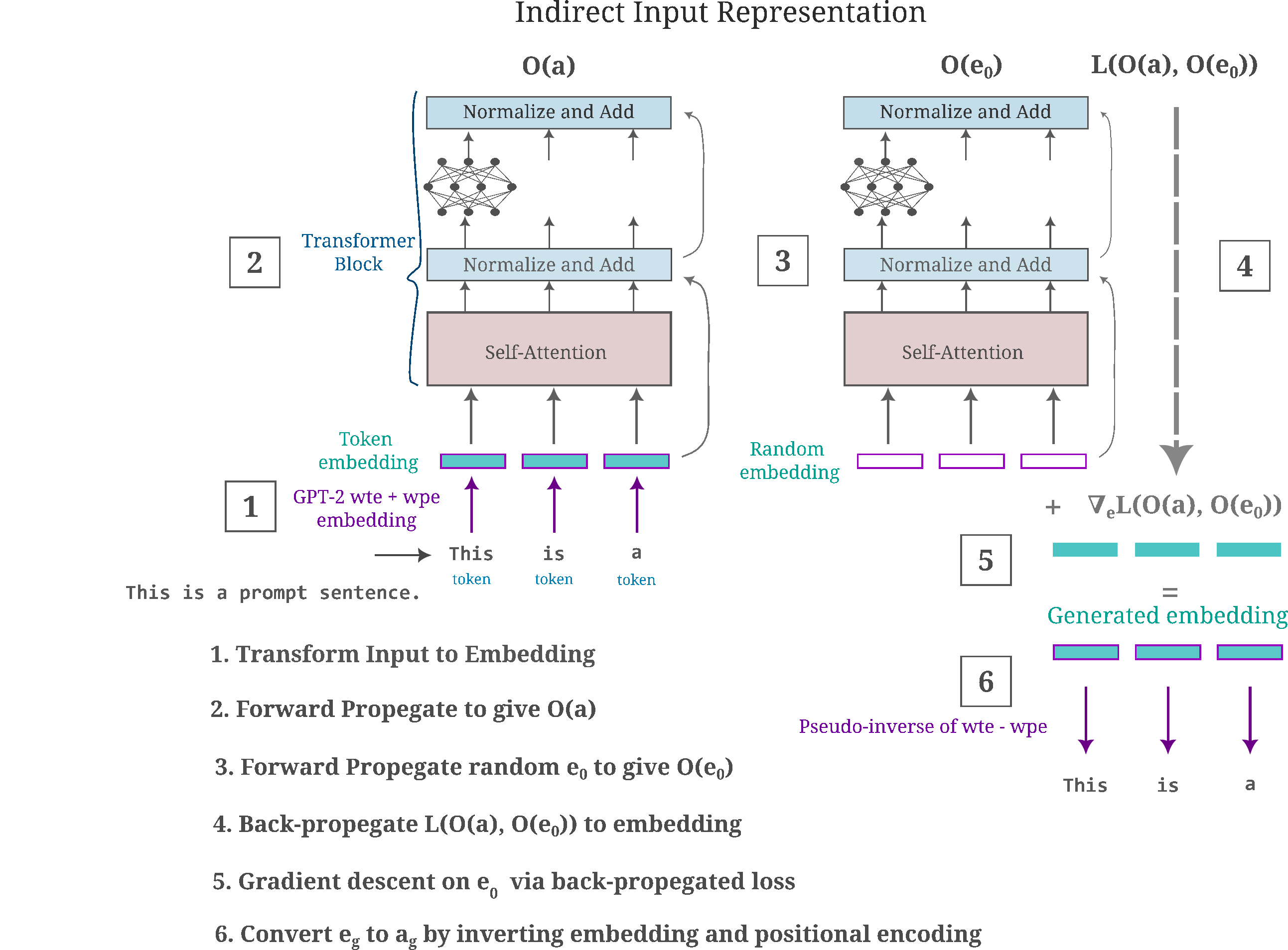
To recap the last section, on this page we will observe the information present in each layer of a given language model by performing gradient descent in embedding space before converting the generated embedding back to tokens. The following figure summarizes how this works for a typical transformer-based model.
One of the primary challenges of large language models today is their ability to generate text that is gramatically and stylistically accurate to the prompt but is inaccurate in some other way, either introducing incorrect information about a topic or else veering off in an unintended direction.
It can be shown, however, that these models are capable of a much more extreme translation from input nonsense into some real language output by making use the the input representations we have generated in the previous section. Suppose one were given the following prompt:
\[\mathtt{The \; sky \; is}\]Feeding this input into a trained GPT-2, we get the very reasonable $\mathtt{blue}$ as the predicted next word. This is clearly one of many possible English texts that may yield that same next word to an accurate language model.
But it can also be shown that one can find many completely nonsensical inputs that also yield an identical output. We will see this first with an untrained version of GPT-2 that has been tructated to include a certain number (below only one) of transformer blocks followed by the language modeling head. The language modeling head allows us to obtain the next predicted word for an input into this model, which provides one measure of ‘closeness’ if our generated sentence has the same next predicted word as the target input.
class AbbreviatedGPT(nn.Module):

	def __init__(self, model):
		super().__init__()
		self.model = model

	def forward(self, x: torch.Tensor):
		# choose the block depth
		for i in range(1):
			x = self.model.transformer.h[i](x)[0]

		x = self.model.lm_head(x)
		return x
When we generate an input after a few hundred iterations of Equation \eqref{eq2}, passing in the resulting embeddings to be inverted by Equation \eqref{eq3} for the target input
\[\mathtt{The \; sky \; is \; blue.}\]we have
\[\mathtt{\; Lime \; Lime \;is \; blueactly} \\ \mathtt{\; enessidateidate \; postp.}\]If an (untrained) language modeling head is attached to this first transformer block, we find that these two inputs really are viewed essentially equivalently for the purposes of causal language modeling, in the sense that the next predicted token for both is $\mathtt{“}$ (for one particular random initialization for GPT-2).
If we increase the number of maximum interations $N$ of our gradient descent procedure in \eqref{eq2} we have
\[\mathtt{\; Terr \; sky \; is \; blue.} \\ \mathtt{\; cyclists \; sky \; is \; blue.}\]And increasing the total iterations $N$ further (to $N \geq 1000$) yields a smaller $L^2$ distance between $a$ and $a_g$ and a greater probability of recovering the original prompt,
\[\mathtt{The \; sky \; is \; blue.}\]although most generated prompts are close but not quite equal to the original for $N = 1000$. Further increasing $N$ leads to more $a_N$ being equivalent to the target $a$. As gradient descent is capable of recovering a target input $a$ across one GPT-2 transformer block this block retains most information on the input, and this recovery is somewhat surprising given that the transformer model is not invertible, such that many inputs may yield an identical output.
With an increase in the number of transformer blocks before the output modeling head, it becomes more difficult to recover the target inptut $a$. For example, many iterations of Equation \eqref{eq2} a model with untrained GPT-2 blocks 1 and 2 we have a generated prompt of
\[\mathtt{The \; sky \; is \; tragedies.}\]Using the full 12 transformer blocks of an untrained (base) GPT-2, followed by the language modeling head (parameters $N=2000, \eta=0.001$), we can recover inputs that yield the same output token as our original prompt but are completely different. For example both $a_g$ of
\[\mathtt{coastline \; DVDs \; isIGHTweak} \\ \mathtt{biologist \; Elephant \; Elephant \; Elephant \; Elephant}\]effectively minimize the $L^1$ distance for different initializations of GPT-2, and yield the same next word (bytecode) token as ‘The sky is blue.’ does.
Language models become less trainable as they are trained
So far we have only considered input representations from untrained models. It may be wondered what the training process does to the model representational ability, and to do so we will use the same abbreviated model configuration above (with GPT-2 transformer blocks following the input and positional embedding and ending in the language modeling head output).
When performing the input representation procedure detailed above on a trained GPT-2 (importantly with a language modeling head attached), the first thing to note is that the model appears to be very poorly conditioned such that using gradient descent to modify an input to match some output requires careful tuning of $\eta$ and many iterations. Indeed it takes a truly enormous number of iterations of \eqref{eq2} to generate $e_g$ such that the model’s output given $e_g$ is closer to the model’s output of $e$ than the slightly shifted input $e’$
\[|| O_l(e_g, \theta) - O_l(e, \theta) ||_1 < || O_l(e', \theta) - O_l(e, \theta) ||_1 \tag{4} \label{eq4}\]on the order to one hundred times as many as for the untrained model to be precise. This very slow minimization of the output loss also occurs when the gradient is calculated on is a different metric, perhaps $L^2$ instead of $L^1$. A quick check shows that there is no change in the general lack of invertibility of even a single GPT-2 transformer module using this metric. Thus it is practically infeasible to make the equality in \eqref{eq4} hold if $e’$ is near $e$ (for example, if $e’ = e + \mathcal{N}(e, \mu=0, \sigma=1/25$).
There is a trivial way to satisfy \eqref{eq4} for any $e’$, and this is to simply make the (formerly random) initial embedding $e_0$ to be equal to the target embedding $e$. Although this is not particularly helpful in understanding the ability of various layers of GPT-2 to represent an input, we can instead make an initial embedding that is a linear combination of random Gaussian noise with the target input.
\[e_0 = s * \mathcal{N}(e, \mu, \sigma) + t * e\]Given an input
\[a = \mathtt{This \; is \; a \; prompt \; sentence.}\]and with $(s, t) = (0.001, 0.999)$ we have at $N=1000$ an $a_g$ such that \eqref{eq4} holds even for $e’$ very close to $e$.
\[\mathtt{interstitial \; Skydragon \; a \; behaviゼウス.}\]Note, however, that even values $(s, t) = (1, 1)$ give an $e_0$ that is capable of being optimized nearly as well as that above, only that more gradient descent iterations are required. For example, the following generated input achieves similar output distance to the input above.
\[\mathtt{opioosponsorsnesotauratedcffff \; conduc}\]Returning to the general case, it takes an extremely large number of iterations of \eqref{eq2} to approach the inequality \eqref{eq4}, and often it cannot be satisfied in a feasible number of iterations at all. This observation suggests that the trained GPT-2 model cannot accurately pass gradients from the output to the input. Why would the gradients arriving at the early layers of a model be inaccurate? It may be wondered if this is due to rounding errors in the backpropegation of gradients. One way to check this is to convert both the model and inputs in question to torch.double() type, ie 64-bit rather than the default 32-bit floating point values. Unfortunately there is no significant change in the number of iterations required to make an input that satisfies \eqref{eq4}, and it remains infeasible to satisfy that inequality for $e’$ very close to $e$.
The relative inability of gradient updates to the input embedding to minimize a loss function on the model output suggests that model layers that are adjacent in the backpropegation computational graph (ie the first few transformer encoders) are also poorly optimized towards the end of training. Indeed, the poor optimization to the input embedding given only one trained transformer block suggests that most of the model is poorly updated towards the end of training, and that only a few output layers are capable of effective updates at this point.
Is there any way to use gradient descent to more effectively minimize some metric distance between a trained model’s output of $a$ versus $a_g$? It turns out that there is: removing the language modeling head reduces the number of iterations required to satisfy \eqref{eq4}, by a factor of $>100$ for a one-block GPT-2 model. This makes it feasible to generate $e_g$ that is accurate even when compared with stricter $e’$ but even these embeddings map to inputs that are more or less completely unrecognizable.
\[\mathtt{srfAttachPsyNetMessage \; Marketable \; srfAttach \; srfAttachPsyNetMessage}\]This result indicates that even when capable of minimizing an $L^1$ metric between $O_l(a, \theta)$ and $O_l(a_g, \theta)$, trained language models still cannot differentiate between gibberish and language. The ability to satisfy \eqref{eq4} once the language modeling head is removed suggests that this head is a kind of gradient bottleneck such that gradient-based optimization becomes much more difficult across the LM head.
Approximate Token Mapping
So far we have seen something somwhat unexpected: given some small input token array $a$ we can recover these tokens from untrained but not trained language model transformer blocks. This indicates that the trained model’s decoder blocks (or the entire model) cannot distinguish between gibberish and a normal sentence. It may be wondered if this is due to the discrete nature of the input: perhaps the $\mathrm{arg \; max}$ of the pseudoinverse of $e_g$ does not find accurate tokens but maybe the second or third highest-activated index could.
We can select the indicies of the top 5 most activated input token positions as follows:
tokens = torch.topk(logits, 5)[1][0] # indicies of topk of tensor
Given
\[\mathtt{This \; is \; a \; prompt \; sentence.}\]For the invertible fully connected network following a token-to-embedding transformation from a trained GPT-2 (as used above) one can see that successive outputs are semantically similar, which is perhaps what one would expect given that a trained embedding would be expected to recover words that mean approximately the same thing (ie ‘speedy’ is an approximate synonym for ‘prompt’). The top five input token strings are
This is a prompt sentence.
 this was an Prompt sentences.(
this are the promptssent,
 This has another speedy paragraph.[
 THIS isna prompted Sent."
but for a non-invertible fully connected model (with layer dims of $[768, 4*768, 768]$) we find that only the top one or two most activated input tokens are recognizable.
 this is a prompt sentence.
thisModLoader an Prompt sentences.–
This corridikumanngthlems.<
 THIS are another guiActiveUnDownloadha Mechdragon
 Thisuberty theetsk recomm.(
The non-invertible model results above are not wholly surprising given that the model used was not trained such that equivalent inputs would not be expected to be very semantically similar. But a model composed of a single trained GPT-2 transformer block (no language modeling head) yields only gibberish as well.
PsyNetMessage▬▬ MarketablePsyNetMessagePsyNetMessagePsyNetMessage
 srfAttachPsyNetMessagePsyNetMessagequerquequerqueartifacts
ocamp��極artifacts��極 unfocusedRange Marketable
irtualquerqueanwhileizontartifactsquerque
Accessorystaking-+-+ザigslistawaru
But when we compare the input representation of one transformer block of a trained model (above) to input representations for one transformer block for a randomly initialized and untrained model (below) we see something interesting: not only does training remove the ability of the first GPT-2 transformer decoder to accurately recover the input sentence from information in the output of that block, but the words corresponding to the input representation of a trained model are much less likely to exist in a real sentence than the decoded input representation by an untrained model. Specifically, observe that Marketable is the only word that would be likely to be ever found in real text above, whereas nearly every word below would likely be found given text of sufficient length.
This together a prompt sentence.
stock PER alotebra benevolentNBC
 estab hydraulic declaration Dyn highlighted Caucas
しFormatorean DAM addressedball
ogeneity shows machine freed erasedcream
This observation suggests that training does indeed confer some ability to distinguish between real sentences: all nearly-sentence representations exhibited by the untrained model are no longer found near the target representation of the trained model, and only inputs that have almost zero probability of appearing in text are observed.
Orthogonal Walk Representations
For the investigation on this page, the main purpose of forming inputs based on the values of the output of some hidden layer is that the input generated gives us an understanding of what kind of information that hidden layer contains. Given a tensor corresponding to output activations of a layer, the information provided by that tensor is typically invariant to some changes in the input such that one can transform one possible input representation into another without changing the output values significantly. The collection of all such invariants may be thought of as defining the information contained in a layer.
Therefore one can investigate the information contained in some given layer by observing what can be changed in the input without resulting in a significant change in the output, starting with an input given in the data distribution. The process of moving along in low-dimensional manifold in higher-dimensional space is commonly referred to a ‘manifold walk’, and we will explore methods that allow one to perform such a walk in the input space, where the lower-dimensional manifold is defined by the (lower-dimensional) hidden layer.
There are a number of approaches to finding which changes in the input are invariant for some model layer output, and of those using the gradient of the output as the source of information there are what we can call direct and indirect methods. Direct methods use the gradient of some transformation on the output applied to the input directly, whereas indirect methods transform the gradient appropriately and apply the transformed values to the input.
We will consider an indirect method first before proceeding to a direct one.
Given the gradient of the output with respect to the input, how would one change the input so as to avoid changing the output? Recall that the gradient of the layer output with respect to the input,
\[\nabla_a O_l(a, \theta)\]expresses the information of the direction (in $a$ space) of greatest increase in (all values of) $O_l(a, \theta)$ for an infinitesmal change. We can obtain the gradient of any layer’s output with respect to the input by modifying a model to end with that layer before using the following method:
def layer_gradient(model, input_tensor):
	...
	input_tensor.requires_grad = True
	output = a_model(input_tensor)
	loss = torch.sum(output)
	loss.backward()
	gradient = input_tensor.grad
	return gradient, loss.item()
If our purpose is to instead avoid changing the layer’s output we want what is essentially the opposite of the gradient, which may be thought of as some direction in $a$-space that we can move such that $O_l(a, \theta)$ is least changed. We can unfortunately not use the opposite of the gradient, as this simply tells us the direction of greatest decrease in $O_l(a, \theta)$. Instead we want a vector that is orthogonal to the gradient, as by definition an infinitesmal change in a direction (there may be many) that is perpendicular to the gradient does not change the output value.
How can we find an orthogonal vector to the gradient? In particular, how may we find an orthogonal vector to the gradient, which is typically a non-square tensor? For a single vector $\mathbf{x}$, we can find an orthogonal vector $\mathbf{y}$ by solving for a solution to the equation of the dot product of these vectors, where the desired product is equal to the zero vector.
\[\mathbf{x} \cdot \mathbf{y} = 0\]We can find that trivially setting $\mathbf{y}$ to be the zero vector itself satisfies the equation, and has minimum norm such that simply finding any solution to the above equation is insufficient for our goals. Moreover, language model input are typically matricies composed of many input tokens embedded such that we want to find vectors that are orthogonal to all input token embedding gradients rather than just one.
To do so, we can make use of the singular value decomposition of the input gradient matrix. Given a matrix $M$ the singular value decomposition is defined as
\[M = U \Sigma V^H\]and may be thought of as an extension of the process of eigendecomposition of a matrix into orthonormal bases to matricies that are non-square. Here the columns of the matrix $U$ is known as the left-singular values of $M$, and the columns of matrix $V$ corresponds to the right-singular values, and $\Sigma$ denotes the singular value matrix that is rectangular diagonal and is analagous to the eigenvalues of an eigendecomposition of a square matrix. $V^H$ denotes the conjugate transpose of $V$, which for real-valued $V$ is $V^H = V^T$.
The singular value decomposition has a number of applications in linear algebra, but for this page we only need to know that if $M$ is real-valued then $U$ and $V$ are real and orthogonal. This is useful because for an $M$ that is non-square, we can find the right-singular values $V$ such that $V^H$ is square. This in turn is useful because some columns (vectors) of $V^H$ are decidedly not orthogonal to $M$ by definition, but as there are more columns in $V^H$ than $M$ we have at least one column that is orthogonal to all columns of $M$.
Now that a number of orthogonal vectors have been obtained, we can update the embedding $e$ to minimize the change in $O_l(e, \theta)$ by
\[e_{n+1} = e_n + \eta * b \left( V^H_{[j+1]} \right)\]where $\eta$ is a sufficiently small update parameter and $j$ indicates the number of tokens in $e$ and $b(V^H)$ indicates a broadcasting of $V^H$ such that the resulting tensor has the same shape as $e_n$, and we repeat for a maximum of $n=N$ iterations. Alternatively, one can assemble a matrix of multiple column vectors of $V^H$ with the same shape as $e$. Empirically there does not appear to be a difference between these two methods.
For example, let’s consider the input
\[\mathtt{The \; sky \; is \; blue.}\]This is a 5-token input for GPT-2, where the embedding corresponding to this input is of dimension $[1, 5, 768]$. Ignoring the first index (minibatch), we have a $5$ by $768$ matrix. If we perform unrestricted singular value decomposition on this matrix and recover $V^H$, we have a $[768, 768]$ -dimension orthogonal matrix. As none of the first $5$ columns of $V^H$ are orthogonal to the columns of $M$ we are therefore guaranteed that the next $763$ columns are orthogonal by definition.
The orthogonal vector approach may therefore be implemented as follows:
def tangent_walk(embedding, steps):
	for i in range(steps):
		embedding = embedding.detach()
		gradient, _ = layer_gradient(a_model, embedding) # defined above
		gradient = torch.squeeze(gradient, dim=0)
		perp_vector = torch.linalg.svd(gradient).Vh[-1] # any index greater than input_length
		embedding = embedding + 0.01*perp_vector # learning rate update via automatically broadcasted vector

	return embedding
where we can check that the SVD gives us sufficiently orthogonal vectors by multiplying the perp_vector by gradient via
print (gradient @ perp_vector) # check for orthogonality via mat mult
If the value returned from this multiplication is sufficiently near zero, the perp_vector is sufficiently orthogonal to the gradient vector and should not change the value of $O_l(a, \theta)$ given an infinitesmal change in $a$ along this direction.
Note that gradients are functions from scalars to vectors (or tensors etc.) rather than functions from vectors to other vectors, meaning that we must actually taking the gradient
\[\sum_i \nabla_a O_l(a, \theta)_i\]which may be implemented as follows:
def individual_gradient(model, input_tensor):
	input_tensor.requires_grad = True
	gradient = torch.zeros(input_tensor.shape).double().to(device)
	output = a_model(input_tensor)
	for i in range(len(output)):
		output = a_model(input_tensor)
		loss = output[i]
		loss.backward()
		gradient += input_tensor.grad
		input_tensor.grad = None

	return gradient
But it is much more efficient to calculate the gradient
\[\nabla_a \sum_i O_l(a, \theta)_i\]which may be implemented as
def summed_gradient(model, input_tensor):
	input_tensor.requires_grad = True
	output = a_model(input_tensor)
	sout = torch.sum(output)
	sout.backward()
	gradient = input_tensor.grad.detach().clone()
	return gradient
It may be empirically verified that Pytorch evaluates these gradients nearly equally, as the difference between the input gradient as calculated by these methods is on the order of $1 \times 10^{-7}$ or less per element.
Equivalently, the above method is computationally identical to
def layer_gradient(model, input_tensor):
	input_tensor.requires_grad = True
	output = a_model(input_tensor)
	output.backward(gradient=torch.ones_like(output).to(device))
	gradient = input_tensor.grad.detach().clone()
	return gradient
This completes the relevant details of the orthogonal walk. Unfortunately this method is not capable of finding new locations in $a$-space that do not change $O(a, \theta)$ significantly. This is due to a number of reasons, the most prominent being that for transformer-based models the perp_vector is usually not very accurately perpendicular to the gradient vector such that multiplication of the orthogonal vector and the gradient returns values on the order of $1 \times 10^{-2}$. This is an issue of poor conditioning inherent in the transformer’s self-attention module leading to numerical errors in the SVD computation, which can be seen by observing that a model with a single transformer encoder yields values on the order of $1 \times 10^{-3}$ whereas a three-layer feedforward model simulating the feedforward layers present in the transformer module yields values on the order of $1 \times 10^{-8}$.
Therefore instead of applying the orthogonal walk approach firectly to the GPT-2 model, we can first apply it to a model architecture that allows the SVD to make accurate orthogonal vectors, the instability of the input gradient landscape makes finite learning rates give significant changes in the output, which we do not want. To gain an understanding for what the problem is, suppose one uses the model architecture mimicking the transformer MLP (with three layers, input and output being the embedding dimension of 768 and the hidden layer 4*768). Obtaining an orthogonal vector from $V^H$ to each token in $e$, we can multiply this vector by $\nabla_a O_l(a, \theta)$ to verify that it is indeed perpendicular. A typical value of this multiplication for the attentionless transformer model block is [ 3.7253e-09, -2.3283e-09, 1.9558e-08, -7.4506e-09, 3.3528e-08], indicating that we have indeed found an approximately orthogonal vector to the gradient for all inputs.
But when we compare the $L^1$ distance metric on the input $d_i =\vert \vert e - e_N \vert \vert_1$ to the same metric on the outputs $d_o =\vert \vert O_l(e, \theta) - O_l(e_N, \theta) \vert \vert_1$ we find that the ratio of output to input distance $d_o / d_i = 2$ when the model used is the three-layer fully connected version. Even using torch.float64 precision, there is typically a larger change in the output than the input although the orthogonal vectors multiplied by the columns of $e$ are then typically on the order of $1 \times 10^{-17}$. After some experimentation, it can be shown that the inefficacy of the orthogonal vector approach is due to the number of elements in the model: for a random initialization of the three-layer MLP for 10 or 50 neurons in the embedding the ratio $d_o / d_i$ is typically $1/2$ or less, but increasing the embedding dimension to $200$ or more leads to the probability of $d_o / d_i < 1$ decreasing substantially.
These results indicate that the orthogonal walk method is not capable of changing the input whilst leaving the output vector unchanged for all except the smallest of models. Nevertheless, for the untrained 3-layer MLP after a few dozen iterations we have
\[\mathtt{\; The \; sky \; is \; blue.} \\ \mathtt{\; and \; sky \; is \; blue.} \\ \mathtt{\; and \; sky \; isadvertisement.} \\ \mathtt{advertisement \; skyadvertisementadvertisement.}\]Although the orthogonal walk method is not particularly successful when applied to GPT-2, we can nevertheless observe a sequence of generated inputs $a_N$ as $n$ increases. One again, however, we do not find inputs of semantic similarity to the desired input.
\[\mathtt{The \; sky \; is \; blue.} \\ \mathtt{confir \; sky \; is \; blue.} \\ \mathtt{\; confir \; behavi \; confir \; confir.}\]When torch.float64 precision is stipulated we find that a much more accurate orthogonal vector may be found, where for any column of the input gradient vector times the right-singular broadcasted vector, $\mathbf g \cdot \mathbf {b(V^H_{[j+1]})}$, is typically on the order of $1 \times 10^{-17}$. Therefore with increased numerical precision we find that computation of the SVD allows one to procure an accurate orthogonal vector to even the poorly conditioned input gradient for GPT-2. But it is remarkable that even for this more accurate orthogonal vector, typically $d_o / d_i > 20$ which means that the orthogonal walk procedure fails spectacularly in finding inputs $a_g$ such that the output is unchanged.
In conclusion, one can walk along a manifold in $a$-space that maps to a unique vector value $O_l(a, \theta)$ by repeated application of a small shift in a direction orthogonal to $\nabla O_l(a, \theta)$, but poor conditioning in this gradient vector means that this method is not capable (at up to 64 bit precision) of an accurate walk (where $O_l(a_n, \theta)$ is nearly identical to the target $O_l(a, \theta)$ for transformer models.
Clamped Gradient Walk Representations
Another approach to changing the input while fixing the output is to clamp portions of the input, add some random amount to those clamped portions, and perform gradient descent on the rest of the input in order to minimize a metric distance between the modified and original output. The gradient we want may be found via
def target_gradient(model, input_tensor, target_output):
	...
	input_tensor.requires_grad = True
	output = a_model(input_tensor)
	loss = torch.sum(torch.abs(output - target_output))
	print (loss.item())
	loss.backward()
	gradient = input_tensor.grad
	return gradient
and the clamping procedure may be implemented by choosing a random index on the embedding dimension and clamping the embedding values of all tokens up to that index, shifting those values by adding these to random normally distributed ones $\mathcal{N}(e; 0, \eta)$. For a random index $i$ chosen between 0 and the number of elements in the embedding $e$ the update rule $f(e) = e_{n+1}$ may be described by the following equation,
\[f(e_{[:, \; :i]}) = e_{[:, \; :i]} + \eta * \mathcal{N}(e_{[:, \; :i]}; 0, \eta) \\ f(e_{[:, \; i:]}) = e_{[:, \; i:]} + \epsilon * \nabla_{e_{[:, \; i:]}} || O_l(e, \theta) - O_l(e^*, \theta) ||_1\]where $e^*$ denotes the original embedding for a given input $a$ and $\eta$ and $\epsilon$ are tunable parameters.
def clamped_walk(embedding, steps, rand_eta, lr):
	with torch.no_grad():
		target_output = a_model(embedding)
	embedding = embedding.detach()

	for i in range(steps):
		clamped = torch.randint(768, (1,))
		shape = embedding[:, :, clamped:].shape
		embedding[:, :, clamped:] += rand_eta*torch.randn(shape).to(device)
		gradient = target_gradient(a_model, embedding, target_output)
		embedding = embedding.detach()
		embedding[:, :, :clamped] = embedding[:, :, :clamped] - lr*gradient[:, :, :clamped]

	return embedding
This technique is far more capable of accomplishing our goal of changing $a$ while leaving $O_l(a, \theta)$ unchanged. For a 12-block transformer model without a language modeling head such that the output shape is identical to the input shape, tuning the values of $\eta, \epsilon, N$ yields an $L^1$ metric on the distance between $m(e, e_N)$ that is $10$ times larger than $m(O_l(e, \theta), O_l(e_n, \theta))$. The ratio $r$ defined as
\[r = \frac{|| e - e_n ||_1} {|| O_l(e, \theta) - O_l(e_N, \theta) ||_1}\]may be further increased to nearly $100$ or more by increasing the number of gradient descent iterations per clamp shift step from one to fifty.
It is interesting to note that the transformer architecture is much more amenable to this gradient clamping optimization than the fully connected model, which generally does not yield an $r>3$ without substantial tuning.
Now that a method of changing the input such that the corresponding change to the output is minimized has been found, we can choose appropriate values of $N, \eta, \epsilon$ such that the $e_N$ corresponds to different input tokens. For successively larger $N$, we have for a trained GPT-2 model (without a language modeling head)
\[\mathtt{elsius \; sky \; is \; blue.} \\ \mathtt{elsius \; skyelsius \; blue.} \\ \mathtt{elsius \; skyelsiuselsius.}\]Once again, we find that the trained GPT-2 approximates an English sentence with gibberish. This is true even if we take the top-k nearest tokens to $e_N$ rather than the top-1 as follows:
elsius skyelsiuselsius.
advertisementelsiusadvertisementascriptadvertisement
eaturesascripteaturesadvertisementelsius
 destroadvertisementhalla blue.]
thelessbiltascript":[{"bilt
Representation Repetitions
It is interesting to note that practically every example of a poorly-formed input representation we have seen on this page suffers from some degree or other of repetition. Take the top-1 token input found above with spaces added for clarity:
\[\mathtt{elsius \; sky \; elsius \; elsius}.\]where $\mathtt{sky}$ is the only target word found and all else are repetitions.
This is interesting in light of the observation that language models (particularly smaller ones) often generate repeated phrases when instructed to give an output of substantial length. This problem is such that efforts have been made to change the output decoding method: for example Su and colleages introduced contrastive search for decoding as opposed to simply decoding the model output as the token with the largest activation (which has been termed a ‘greedy’ decoding approach) during autoregression.
The tendancy language models tend to generate repetitive text during autoregression has been attributed by Welleck and colleages to the method by which language models are usually trained, ie maximum likelihood on the next token in a string. The authors found that two measures ameliorate this repetition: modifying the objective function (‘maximum unlikelihood estimation’) and modifying the decoding method to instead perform what is called a beam search. For all inputs $a$ of some dataset where each input sequence is composed of tokens $a = (t_0, t_1, t_2, …, t_n)$ where the set of all possible tokens $T$ such that $t_n \in T$, minimization of the log-likelihood of the next token $t_i$ may be expressed as
\[t_i = \underset{t_i}{\mathrm{arg \; min}} \; - \sum_a \sum_{T} \log p(t_i | O(t_{i-1}, t_{i-2}, ..., t_1; \; \theta))\]Beam search instead attempts to maximize the total likelihood over a sequence of tokens rather than just one. For two tokens, this is
\[t_i, \; t_{i-1} = \underset{t_i, \; t_{i-1}}{\mathrm{arg \; min}} \; - \sum_a \sum_{T} \log p(t_i, t_{i-1} | O(t_{i-2}, t_{i-3}, ..., t_1; \; \theta))\]where $t_{i-1}$ may be any of the number of beams specified. A good explanation of beam search relative to topk or other methods may be found here.
Returning to our model representation findings, it is clear that GPT-2 indeed tends to be unable to distinguish between repetitive sequences and true sentences. But viewed through the lense of representation theory, there is a clear reason why this would be: training has presumably never exposed the model to a sequence like $\mathtt{elsius \; sky \; elsius \; elsius}.$ as the training inputs are generally gramatically correct sentences. Therefore there is no ‘hard’ penalty on viewing these nonsensical phrases as being identical to real ones, in the sense that the loss function would not necessarily have placed a large penalty on a model that generates this phrase.
On the other hand, it is also clear that there is indeed some kind of penalty placed on this phrase because it should never appear during training. This is analagous to the idea of opportunity cost in economics, in which simply not choosing a profitable activity may be viewed as incurring some cost (the lost profit). Here a model that generates a nonsensical phrase is penalized in the sense that this output could not possibly give the model any benefit with regards to maximum likelihood training on the next token, whereas even a very unlikely but gramatically correct phrase could appear in some text and therefore could be rewarded.
Equivalently, observe that a model that has effectively minimized its log-likelihood objective function should not repeat words or phrases unless such repetitions were found in the training data, as errors such as these (on a per-token basis) would necessarily increase the negative log-likelihood. Therefore all language models of sufficiently high capacity, when trained on enough data are expected to avoid repetition.
These observations suggest that if one were to train a language model of sufficiently large capacity on a sufficiently large dataset, repetition would cease to be found as this model would more effectively minimize negative log-likelihood. From the performance of more recent and larger models than GPT-2 we can see that this may indeed be correct. Does this mean that the representation in larger models trained on more data will also be less prone to repetition?
The first part of this question answered by performing the same input representation procedure on larger versions of GPT-2, where the models have been trained on the same dataset (40 GB of text from Reddit links mostly). On this page we have thus far considered the base GPT-2 model with 117M parameters, and now we can observe the input representation repetition for the gpt2-xl with 1.6B parameters. Once we have downloaded the appropriate trained models from the HuggingFace transformers store, which for gpt2-xl may be done as follows:
from transformers import AutoTokenizer, AutoModelForCausalLM

tokenizer = AutoTokenizer.from_pretrained("gpt2")
model = AutoModelForCausalLM.from_pretrained("gpt2-xl")
we find that optimizing an input to match the output of the first transformer block is perhaps easier than it was for the gpt2-base model with a tenth of the parameters, where a mere 20 iterations of gradient descent is more than enough to satisfy the desired inequality in which the measure of distance between the generated input’s output is smaller than the shifted input’s output as described in \eqref{eq4}.
".[.>>.–.–.–
ADA.–annabin.>>.>>
kus".[ADAwanaiannopoulos
iott Gleaming.>>".[olor
 Gleamingoloriottiannopouloswana
Interestingly, however, we can see that there is now much less repetition for each topk decoding. The same is true if we use the first 12 transformer decoders, which yield a top5 input representation as follows:
iets largeDownloadnatureconservancy".[twitter
udeauhexDonnellramids".[
 largeDownload2200ledgePsyNetMessage>[
retteimanclipsTPPStreamerBot王
 Citizenudeau2200brycekson
and for a 24-block hidden architecture the top5 decodings of the input representation are
 Marketable (" Dragonboundju.>>
ossessionoptimisoliband().
minecraftsocketramid,...!.
iczisphere Canyonpiresaer
eloowntgur Pastebinnatureconservancy
and even for 40 blocks,
iczisphere Dragonboundheit\
umerableaddonszoneNT>.
auerohnramidohlSTEM
ozisonssoleolin.<
uskyankaFSibandrawl
The author’s local GPU (an RTX 3060 with 12GB memory) runs out of memory trying to perform backpropegation on the full 48-block gpt2-xl. In this case we are faced with a few options: either we can use larger GPUs or else we can compress the model or model’s parameters in some way. Model parameters are usually set to a 32-bit floating point datatype by default, but for this input representation visualization process we do not actually need full precision. Instead, we can load and convert the model to (mostly) 8-bit precision using Tim Dettmer’s very useful bitsandbytes library (or the ported bitsandbytes-windows version if you are using Windows), which is integrated into the AutoModelForCausalLM module in the Huggingface Transformers library such that a model may be loaded to a GPU in 8 bit precision using the following:
model = AutoModelForCausalLM.from_pretrained("gpt2-xl", load_in_8bit=True, device_map='auto')
bitsandbytes does not actually convert all model parameters to 8-bit precision due to the ubiquitous presence of outlier features in large language models, as shown by Dettmers and colleages. Note that most CPUs do not support linear algebraic operations with any datatype less than 32 bits, so a GPU should be used here. Once the model has been loaded, for the full 48-block stack of GPT-2 we have a top-5 representation of the input ‘The sky is blue.’ represented as
 COURisphere Dragonboundheit\<
=>addonsGWolin>.
umerableankaOrgNTrawl
CVE '[soleiband.<
fter ('ramidohl$.
It is interesting to note that gradient-based optimization of the input is much more difficult for the full 48-block GPT-2 than even first 24-block subset of this model, indicating that the later transformer blocks are poorly conditioned relative to the earlier blocks. This is true even when 8-bit quantization is performed on the smaller subsets, indicating that quantization is not in this case responsible for difficulties optimizing via gradient descent.
To summarize this last section, simply increasing the model’s size does seem to reduce the amount of repetition, but even the larger models we have investigated thus far do not exhibit accurate representations of language inputs. This investigation is continued in Part III.
Implications
In summary, transformer-based language models in the GPT-2 family are unable to distinguish between real English sentences and pure gibberish. Given a point in a transformer block hidden layer space corresponding to an input of a real sentence, we have found that most nearby points correspond to inputs that are not even approximately sentences but are instead completely unintelligible.
There exists a notable difference between trained language and vision transformer models: the latter contain modules that are at least partially capable of discerning what the input was composed of, whereas the latter does not. But when we consider the training process for language models, it is perhaps unsurprising that input representations are relatively poor. Note that each of the gibberish input generations were almost certainly not found in the training dataset precisely because they are very far from any real language. This means that the language model has no a priori reason to differentiate between these inputs and real text, and thus it is not altogether unsurprising that the model’s internal representations would be unable to distinguish between the two.
In a sense, it is somewhat more unexpected that language models are so poorly capable of approximate rather than exact input representation. Consider the case of one untrained transformer encoder detailed in a previous section: this module was unable to exactly represent the input (for the majority of random initializations) but the representations generated are semantically similar to the original prompt. This is what we saw for vision models, as input representations strongly resembled the target input even if they were not exact copies. The training process therefore results in the loss of representational accuracy from the transformer encoders.
In this page’s introduction, we considered the implications of the ‘no free lunch’ theorems that state (roughly) that no on particular model is better than any others at all possible machine learning tasks. Which tasks a given model performs well or poorly on depends on the model architecture and training protocol, and on this page we saw that trained language models perform quite poorly at the task of input generation because even early layers are unable to differentiate between English sentences and gibberish. Non-invertibility alone does not explain why these trained models are poor discriminators, but the training protocol (simply predicting the next word in a sentence) may do so.
When one compares the difference in vision versus language transformer model input representational ability, it is clear that language models retain much less information on their inputs. But when we consider the nature of language, this may not be altogether surprising: language places high probability on an extraordinarily small subset of possible inputs relative to natural images. For example, an image input’s identity is invariant to changes in position, orientation (rotation), order, smoothness (ie a grainy image of a toaster is still a toaster), and brightness. But a language input is not invariant to any of these transformations. A much smaller subset of all possible inputs (all possible word or bytecode tokens in a sequence) are therefore equivalent to language models, and the invariants to be learned may be more difficult to identify than for vision models.
Finally, it is also apparent that it is much more difficult to optimize an input via gradient descent on the loss of the model output after training versus before. This appears to be a somewhat attention-intrinsic phenomenon and was also observed to be present in Vision Transformers, but we find that language modeling heads (transformations from hidden space to output tokens) are particularly difficult to optimize across. This observations suggests that efficient training of transformer-based models is quite difficult, and could contribute to the notoriously long training time required for large language models. Freezing the language modeling head transformation would therefore be expected to assist the training process.