Representation in Vision Transformers and Attentionless Models

Introduction

The convolutional neural network has been the mainstay of deep learning vision approaches for decades, dating back to the work of LeCun and colleagues in 1989. In the that work, it was proposed that restrictions on model capacity would be necessary to prevent over-parametrized fully connected models from failing to generalize and that these restrictions (translation invariance, local weight sharing etc.) could be encoded into the model itself.

Convolution-based neural networks have since become the predominant deep learning method for image classification and generation due to their parsimonius weight sharing (allowing for larger inputs to be modeled with fewer parameters than traditional fully connected models), their flexibility (as with proper pooling after convolutional layers a single model may be applied to images of many sizes), and above all their efficacy (nearly every state-of-the-art vision model since the early 90s has been based on convolutions).

It is interesting to note therefore that one of the primary motivations of the use of convolutions, that over-parametrized models must be restricted in order to avoid overfitting, has since been found to not apply to deep learning models. Over-parametrixed fully connected models do not tend to overfit image data even if they are capable of doing so, and furthermore convolutional models that are currently applied to classify (quite accurately too) large image dataasets are capable of fitting pure noise (ref).

Therefore it is reasonable to hypothesize that the convolutional architecture, although effective and flexible, is by no means required for accurate image classification or other vision tasks. One particularly effective approach has been translated from the field of natural language processing that has been termed the ‘transformer’, which makes use of self-attention mechanisms. We also consider mlp-based mixer architectures that do not make use of attention.

Transformer architecture

We focus on the ViT B 32 model introduced by Dosovitsky and colleagues. This model is based on the original transformer from Vaswani and colleages, in which self-attention modules previously applied with recurrent neural networks were instead applied to patched and positionally-encoded sequences in series with simple fully connected architectures.

The transformer architecture was found to be effective for natural language processing tasks and was subsequently employed in vision tasks after convolutional layers. But the work introducing the ViT went further and applied the transformer architecture directly to patches of images, which has been claimed to occur without explicit convolutions (but does in fact used strided convolution to form patch embeddings as we will later see). It is an open question of how similar these models are to convolutional neural networks.

The transformer is a feedforward neural network model that adapted a concept called ‘self-attention’ from recurrent neural networks that were developed previously. Attention modules attempted to overcome the tendancy of recurrent neural networks to be overly influenced by input elements that directly preceed the current element and ‘forget’ those that came long before. The original transformer innovated by applying attention to tokens (usually word embeddings) followed by an MLP, foregoing the time-inefficiencies associated with recurrent neural nets.

In the original self-attention module, each input (usually an embedding of a word) is associated with three vectors $k, q, v$ for Key, Query, and Value that are produced from multiplying learned weight matricies $W^K, W^Q, W^V$ to the input $X$. Similarity between inputs to the first element (denoted by the vector $\pmb{s_1}$) is calculated by finding the dot product (denoted $\cdot$) of one element’s query vector with all element’s key vectors as follows:

\[\pmb{s_1} = (q_1 \cdot k_1, q_1 \cdot k_2, q_1 \cdot k_3,...)\]

before constant scaling followed by a softmax transformation to the vector $\pmb{s_1}$ to make $\pmb{s_1’}$. Finally each of the resulting scalar components of $s$ are multiplied by the corresponding value vectors for each input $v_1, v_2, v_3,…$ and the resulting vectors are summed up to make the activation vector $\pmb{z_1}$ (that is the same dimension as the input $X$ for single-headed attention).

\[\pmb{s_1'} = \mathbf{softmax} \; ((q_1 \cdot k_1)/\sqrt d, (q_1 \cdot k_2)/ \sqrt d, (q_1 \cdot k_3)/ \sqrt d,...) \\ \pmb{s_1'} = (s_{1,1}', s_{1,2}', s_{1,3}',...) \\ \pmb{z_1} = v_1 s_{1,1}' + v_2 s_{1,2}' + v_3 s_{1,3}'+ \cdots + v_n s_{1,n}\]

The theoretical basis behind the attention module is that certain tokens (originally word embeddings) should ‘pay attention’ to certain other tokens moreso than average, and that this relationship should be learned directly by the model. For example, given the sentence ‘The dog felt animosity towards the cat, so he behaved poorly towards it’ it is clear that the word ‘it’ should be closely associated with the word ‘cat’, and the attention module’s goal is to model such associations.

When we reflect on the separate mathematical operations of attention, it is clear that they do indeed capture something that may be accurately described by the English word. In the first step of attention, the production of $q, k, v$ vectors from $W^K, W^Q, W^V$ weight matricies can be thought of as projecting the input embedding $X$ into the relevant vectors such that something useful about the input $X$ is captured, being that these weight matricies are trainable parameters. The dot product between vectors $q_1$ and $k_2$ may be thought of as a measure of the similarity between embeddings 1 and 2 precisely because the dot product itself may be understood as a measure of vector similarity: the larger the value of $q_1 \cdot k_2$, the more similar these entities are assuming similar norms among all vectors $q, k$. Softmax then normalizes attention such that all values $s$ are between 0 (least attention) and 1 (most attention). The process of multiplying these attention values $s$ by the value vectors $v$ serves to ‘weight’ these value vectors based on that attention amount. If the value vectors accurately capture information in the input $X$, then the attention module yields an output that is a additive combination of $v$ but with the ‘most similar’ (ie largest $s$) $v$ having the largest weight.

But this clean theoretical justification breaks down when one considers that models with single attention modules generally do not perform well on their own but require many attention modules in parallel (termed multi-head attention) and in series. Given a multi-head attention, one might consider each separate attention value to be context-specific, but it is unclear why then attention should be used at all given that an MLP alone may be thought of as providing context-specific attention. Transformer-based models are furthermore typically many layers deep, and it is unclear what the attention value of an attention value of a token actually means.

Nevertheless, to gain familiarity with this model we note that for multi-head attention, multiple self-attention $z_1$ vectors are obtained (and thus multiple key, value, and query weight matricies $W^K, W^Q, W^V$ are learned) for each input. The multi-head attention is usually followed by a layer normalization and fully connected layer (followed by another layer normalization) to make one transformer encoder. Attention modules are serialized by simply stacking multiple encoder modules sequentially.

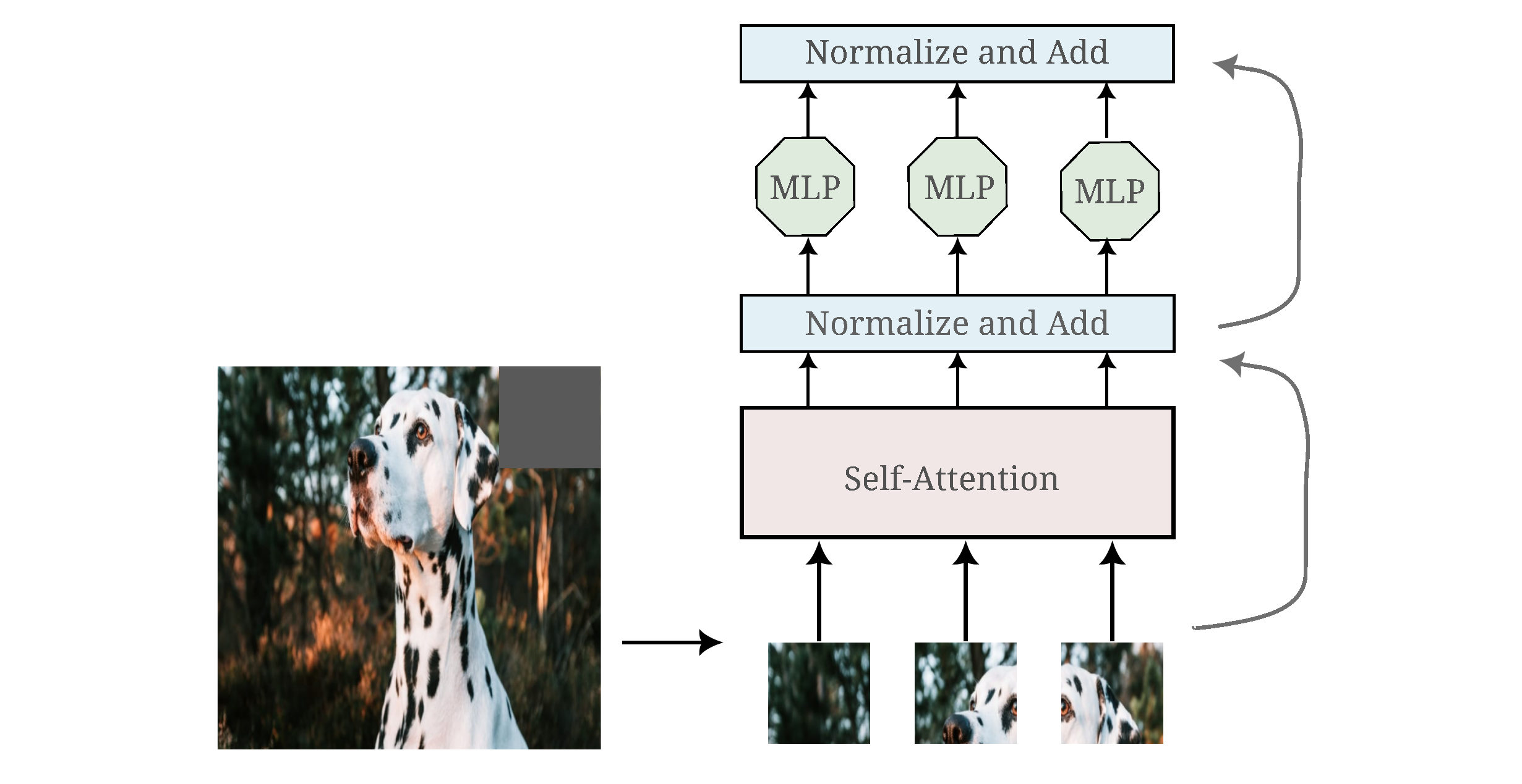
A single transformer encoder applied to image data may be depicted as follows:

For a more thorough introduction to the transformer, see Alammar’s Illustrated Transformer. See here for an example of a transformer encoder architecture applied to a character sequence classification task.

Input Generation with Vision Transformers

One way to understand how a model yields its outputs is to observe the inputs that one can generate using the information present in the model itself. This may be accomplished by picking an output class of interest (here the models have been trained on ImageNet so we can choose any of the 1000 classes present there), assigning a large constant to the output of that class and then performing gradient descent on the input, minimizing the difference of the model’s output given initial random noise and that large constant for the specified output index.

We add two modifications to the technique denoted in the last paragraph: a 3x3 Gaussian convolution (starting with $\sigma=2.4$ and ending with $sigma=0.$) is performed on the input after each iteration and after around 200 iterations the input is positionally jittered using cropped regions. For more information see this page.

More precisely, the image generation process is as follows: given a trained model $\theta$ we construct an appropriately sized random input $a_0$

\[a_0 = \mathcal{N}(a; \mu=0.7, \sigma=1/20)\]

next we find the gradient of the absolute value of the difference between some large constant $C$ and the output at our desired index $O(a_0, \theta)_i$ with respect to that random input,

\[g = \nabla_{a_0} |C - O(a_0, \theta)_i|\]

and finally input is updated by gradient descent followed by Gaussian convolution $\mathcal{N_c}$

\[a_{n+1} = \mathcal{N_c}(a_n - \epsilon * g)\]

Positional jitter is applied between updates such that the subset of the input $a_n$ that is fed to the model undergoes gradient descent and Gaussian convolution, while the rest of the input is unchanged.

\[a_{n+1[:, \;m:n, \;o:p]} = \mathcal{N_c}(a_{n[:, \; m:n, \; o:p]} - \epsilon * \nabla_{a_{n}[:, \; m:n, \;o:p]} |C - O(a_{n[:, \; m:n, \; o:p]}, \theta)_i|)\]

One of the first differences of note compared to the inputs generated from convolutional models is the lower resolution of the generated images: this is partly due to the inability of vision transformer base 32 (ViT B 32) to pool outputs before the classification step such that all model inputs must be of dimension $3x224x224$, whereas most convolutional models allow for inputs to extend to $3x299x299$ or even beyond $3x500x500$ due to max pooling layers following convolutions.

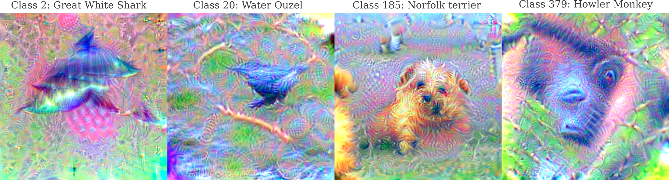
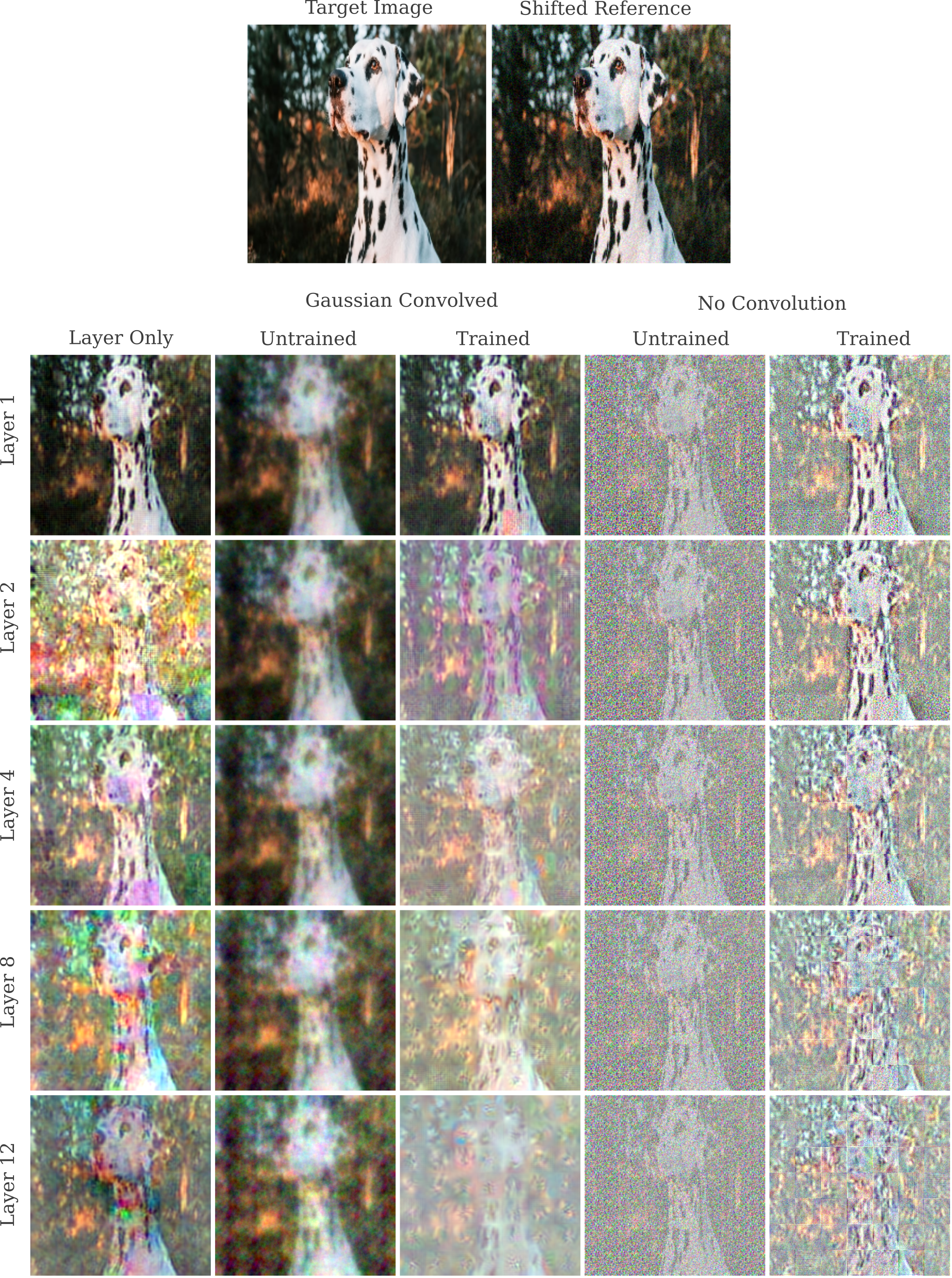
When we observe representative images of a subset of ImageNet animal classes with Vit B 32,

as well as landscapes and inanimate objects with the same model,

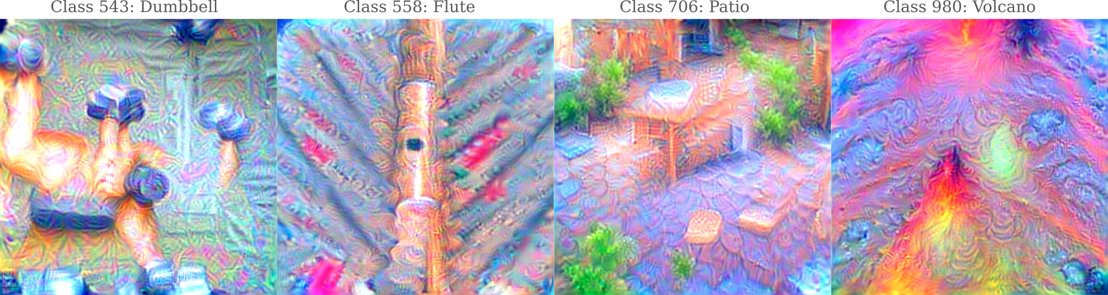
it is clear that recognizable images may be formed using only the information present in the vision transformer architecture just as was accomplished for convolutional models.

Vision Transformer hidden layer representation overview

Another way to understand a model is to observe the extent to which various hidden layers in that model are able to autoencode an input: the better the autoencoding, the more complete the information in that layer.

First, let’s examine an image that is representative of one of the 1000 categories in the ImageNet 1k dataset: a dalmatian. We can obtain various layer outputs by subclassing the pytorch nn.Module class and accessing the original vision transformer model as self.model. For ViT models, the desired transformer encoder layer outputs may be accessed as follows:

class NewVit(nn.Module):

    def __init__(self, model):
        super().__init__()
        self.model = model
    
    def forward(self, x: torch.Tensor, layer: int):
        # Reshape and permute the input tensor
        x = self.model._process_input(x)
        n = x.shape[0]

        # Expand the class token to the full batch
        batch_class_token = self.model.class_token.expand(n, -1, -1)
        x = torch.cat([batch_class_token, x], dim=1)
        for i in range(layer):
            x = self.model.encoder.layers[i](x)
        return x

where layer indicates the layer of the output desired (self.model.encoder.layers are 0-indexed so the numbering is accurate). The NewVit class can then be instantiated as

vision_transformer = torchvision.models.vit_b_32(weights='IMAGENET1K_V1')
new_vision = NewVit(vision_transformer).to(device)
new_vision.eval()

First let’s observe the effect of layer depth (specifically transformer encoder layer depth) on the representation accuracy of an untrained ViT_B_32 and compare this to what was observed for ResNet50 (which appears to be a fairly good stand-in for other convolutional models).

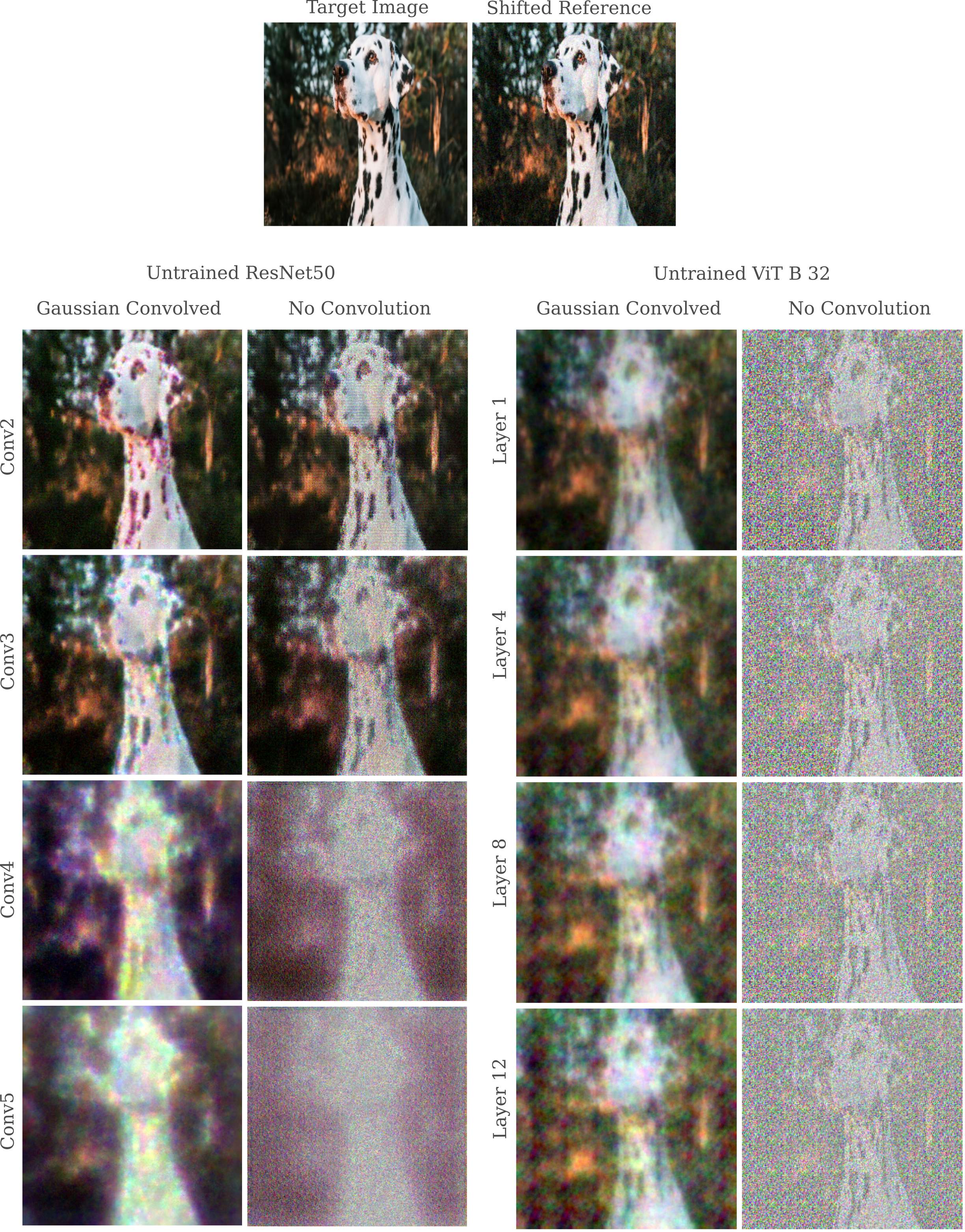
The first notable aspect of input representation is that it appears to be much more difficult to approximate a natural image using Gaussian-convolved representations for ViT than for ResNet50, or more precisely it is difficult to find a learning rate $\epsilon$ such that the norm of the difference between the target output $O(a, \theta)$ and the output of the generated input $O(a_g, \theta)$ is smaller than the norm of the difference between the target output and the output of a slightly shifted input $O(a’, \theta)$ where $a’ = a + \mathcal{N}(a; \mu=0, \sigma=1/18)$, meaning that it is difficult to obtain the following inequality:

\[||O(a, \theta) - O(a', \theta)||_2 < ||O(a, \theta) - O(a_g, \theta)||_2\]

Compare the decreasing representation clarity with increased depth to the nearly constant degree of clarity in the ViT: even at the twelth and final encoder, the representation quality is approximately the same as that in the first layer. The reason as to why this is the case is explored in the next section.

As each encoder is the same size, we can also observe the representation of only that encoder (rather than the given encoder and all those preceeding it).

ViT input processing convolutions are nonoptimal

When we consider the representation of the first layer of the vision transformer compared to the first layer in ResNet50, it is apparent that the former has a less accurate representation. Before this first layer, ViT has an input processing step in which the input is encoded as a sequence of tokens, which occurs by forming 768 convolutional filters each 3x32x32 (hence the name ViT B 32) large, with 32-size strides. In effect, this means that the model takes 32x32 patches (3 colors each) of the original input and encodes 768 different 3x7x7 arrays which act analagously to the word embeddings used in the original transformer.

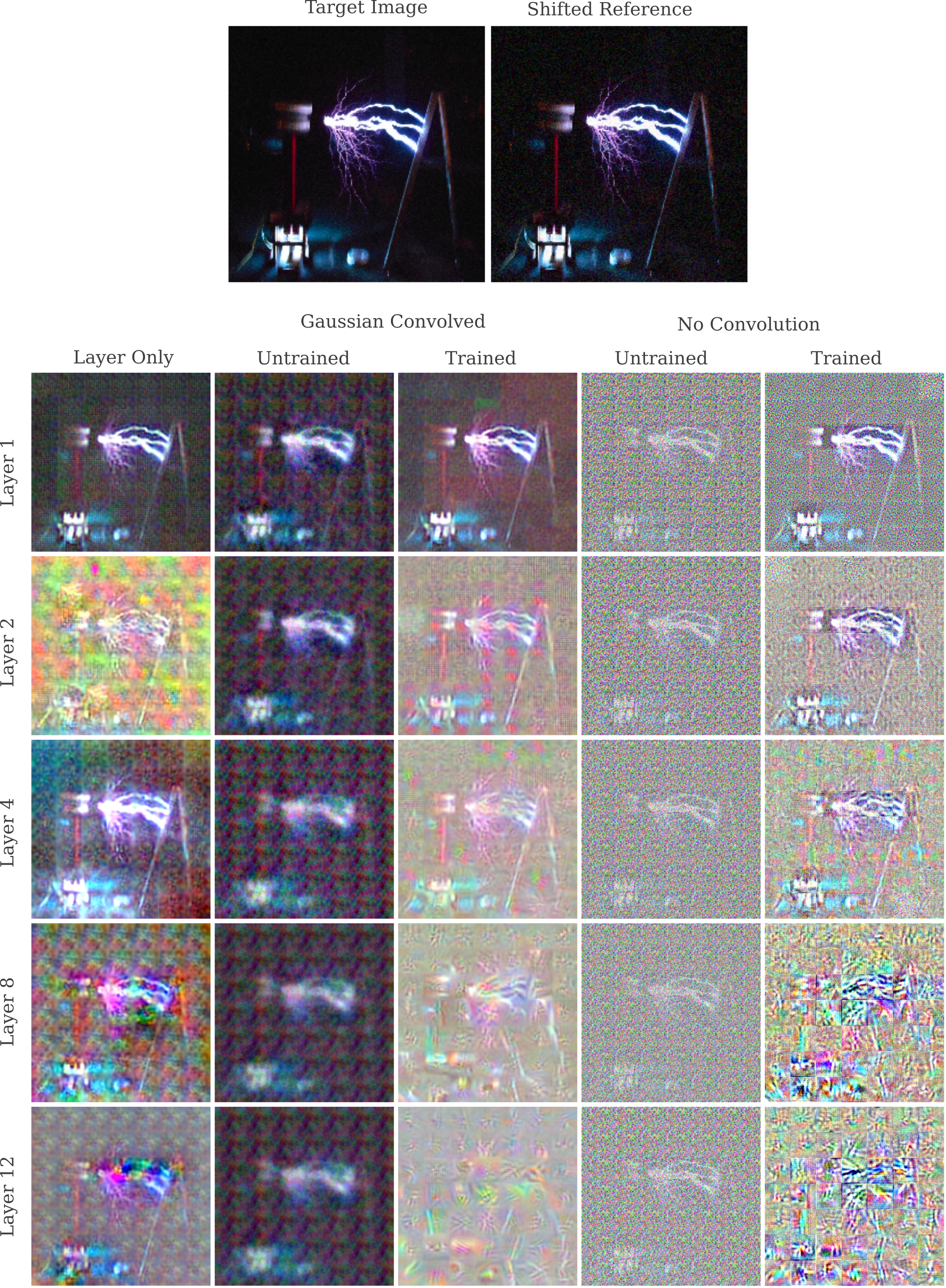
It may be wondered then if it is the input processing step via strided 32x32 convolutions or the first encoder layer that is responsible for the decrease in representation accuracy. Generating representation of the outputs of first the input processing convolution and then the input processing followed by the first encoder layer of an initial image of a tesla coil, it is clear that the input processing itself is responsible for the decreased representation clarity, and furthermore that training greatly enhances the processing convolutional layer’s representation resolution (although still not to the degree seen in the first convolution of ResNet)

For ResNet50, an increase in representation resolution for the first convolutional layer upon training is observed to coincide with the appearance of Gabor function wavelets in the weights of that layer (see the last supplementary figure of this paper). It may be wondered if the same effect of training is observed for these strided convolutions, and so we plot the normalized (minimum set to 0, maximum set to 1, and all other weights assigned accordingly) weights before and after training to find out.

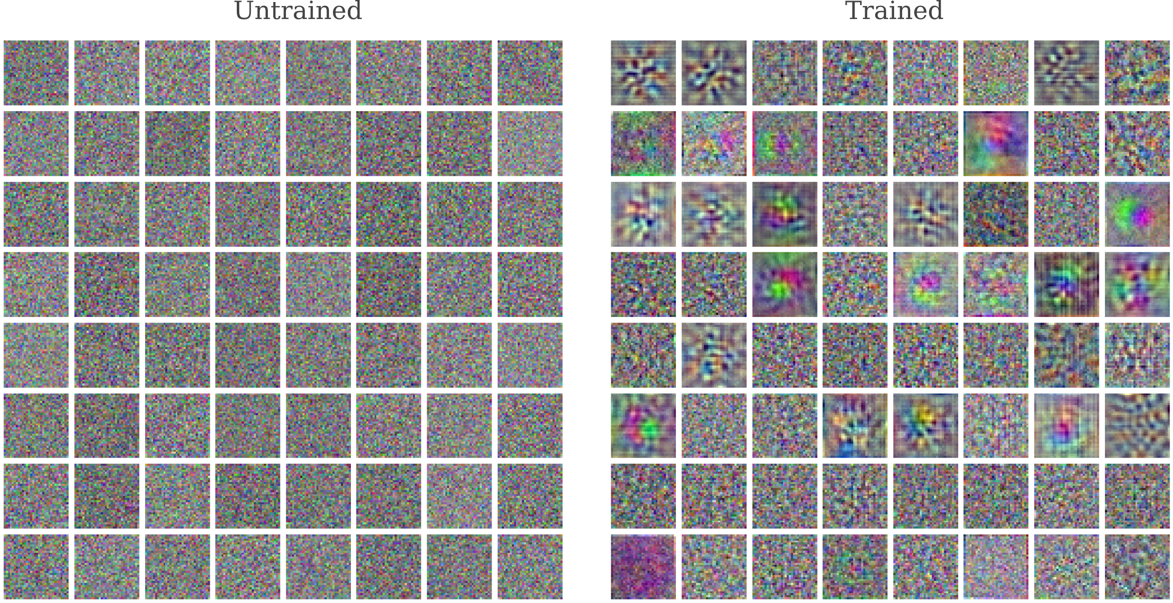
In some convolutions we do indeed see wavelets (of various frequencies too) but in other we see something curious: no discernable pattern at all is visible in the weights of around half of the input convolutional filters. As seen in the paper referenced in the last paragraph, this is not at all what is seen for ResNet50’s first convolutional layer, where every convolutional filter plotted has a markedly non-random weight distribution (most are wavelets).

Earlier it was observed that for Vit B 32 the process of training led to the appearance of wavelet patterns in the input convolution layer and a concomitant increase in representational accuracy. For that model the convolutional operation is not overcomplete, but for the ViT Large 16 model it is. It can therefore be hypothesized that training is not necessary for accurate input representation for the procesing convolution of ViT L 16, and indeed this is found to be the case.

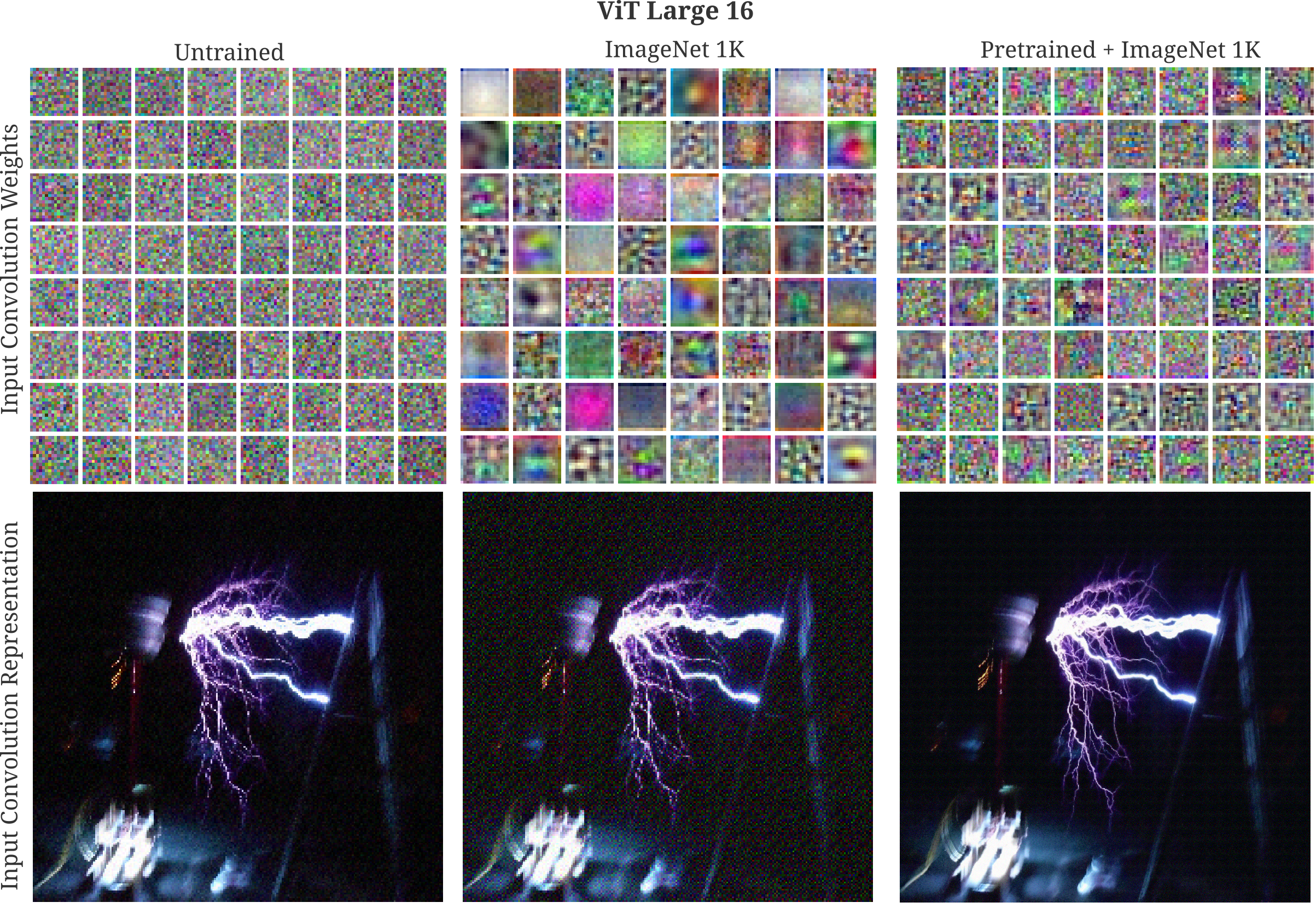
Note the lack of consistent wavelet weight patterns in the input convolution, even after training (and even after extensive pretraining on weakly supervised). This observation may explain why Xaio and colleagues found that replacing the strided input processing convolutions above with 4 layers of 3x3 convolutions (followed by one 1x1 layer) improves vision transformer training stability and convergence as well as ImageNet test accuracy.

Poor Input representation from untrained layer normalization

Being that the input convolutional stem to the smaller ViT models is not capable of accurately representing an input, to understand later layers’ representation capability we can substitute a trained input processing convolutional layer from a trained vision transformer, and chain this layer to the rest of a model from an untrained ViT.

class NewVit(nn.Module):

    def __init__(self, model):
        super().__init__()
        self.model = model
    
    def forward(self, x: torch.Tensor):
        # Apply a trained input convolution
        x = trained_vit._process_input(x)
        n = x.shape[0]

        # Expand the class token to the full batch
        batch_class_token = self.model.class_token.expand(n, -1, -1)
        x = torch.cat([batch_class_token, x], dim=1)
        for i in range(1):
            x = self.model.encoder.layers[i](x)
            
vision_transformer = torchvision.models.vit_h_14().to(device) # untrained model
trained_vit = torchvision.models.vit_h_14(weights='DEFAULT').to(device) # weights='IMAGENET1K_V1'
trained_vit.eval()
new_vision = NewVit(vision_transformer).to(device)
new

When various layer representations are generated for ViT Base 32, it is clear that although there is a decrease in representation accuracy as depth increases in the encoder stack with fixed ($n=1,500$) iterations, this is mostly due to approximate rather than true non-invertibility as increasing the number of iterations of the generation process to $n=105,000$ yields a representation from the last encoder layer that is more accurate than that obtained with fewer iterations from the first.

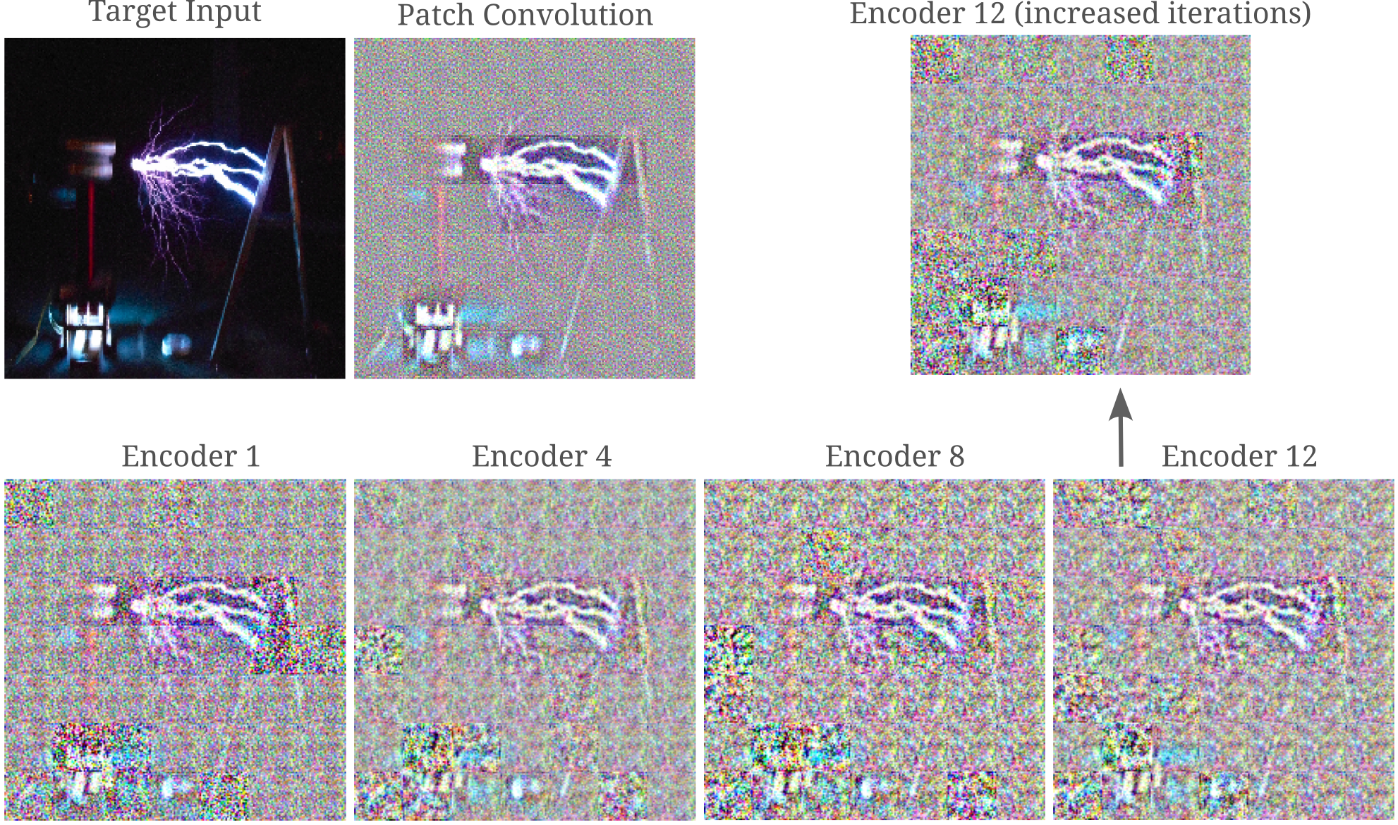
It is apparent that all encoder layers have imperfections in certain patches, making them less accurate than the input convolution layer’s representation. It may be wondered why this is, being that the encoder layers have outputs of dimension $50x768$ which is slightly larger than the input convolutional output of $49x768$ due to the inclusion of a ‘class token’ (which is a broadcasted token that is used for the classification output).

Vision transformer models apply positional encodings to the tokens after the input convolution in the first transformer encoder block, and notably this positional encoding is itself trained: initialized as a normal distribution nn.Parameter(torch.empty(1, seq_length, hidden_dim).normal_(std=0.02)), this positional encoding tensor (torch.nn.Parameter objects are torch.Tensor subclasses) is back-propegated through such that the tensor elements are modified during training. It may be wondered if a change in positional encoding parameters is responsible for the change in first encoder layer representational accuracy. This can be easily tested: re-assigning an untrained vision transformer’s positional embedding parameters to that of a trained model’s positional embedding parameters may be accomplished as follows:

vision_transformer = torchvision.models.vit_b_32(weights='DEFAULT').to(device) # 'IMAGENET1K_V1'
vision_transformer.eval()
untrained_vision = torchvision.models.vit_b_32().to(device)
untrained_vision.encoder.pos_embedding = vision_transformer.encoder.pos_embedding

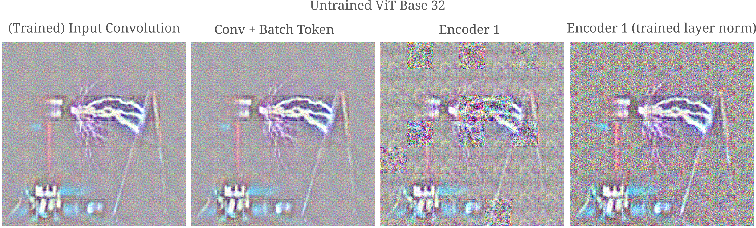
When this is done, however, there is no noticeable difference in the representation quality. Repeating the above procedure for other components of the first transformer encoder, we find that substituting the first layer norm (the one that is applied before the self-attention module) of the first encoder for a trained version is capable of increasing the representational quality substantially.

Layer Normalization considered

In the last section it was observed that changing the parameters (specifically swapping untrained parameters for trained ones) of a layer normalization operation led to an increase in representational accuracy. Later on this page we will see that layer normalization tends to decrease representational accuracy, and so we will stop to consider what exactly this transformation entails.

Given a layer’s features indexed by $n$ with the layer’s activations denoted $x_n$, the output of layer normalization $y$ is defined as

\[y = \frac{x - \mathrm{E}(x_n)}{\sqrt{\mathrm{Var}(x_n) + \epsilon}} * \gamma + \beta\]

where $\gamma$ and $\beta$ are trainable parameters. Here the expectation $\mathrm{E}(x_n)$ refers to the mean of certain dimensions of $x$, termed features, and variance $\mathrm{Var}(x)$ is the sum-of-squares variance on those same dimensions. For transformer models, features are typically the activations of each neuron in the MLP of each block, meaning that layer normalization as it is applied to vision transformers most accurately normalizes values in each image patch separately.

Short consideration of the above formula should be enough to convince one that layer normalization is in general non-invertible such that many different possible inputs $x$ may yield one identical output $y$ for any $\gamma, \beta$ values. For example, observe that $x = [0, 2, 4]^T, t = [-1, 0, 1]^T, u = [2.1, 2.2, 2.3]^T$ are all mapped to the same $y$ despite having very different $\mathrm{Var}(x)$ and $\mathrm{E}(x)$ and elementwise values in $x$.

Thus it should come as no surprise that the vision transformer’s representations of the input often form noticeably patchwork-like images when layer normalization is applied (to each patch separately). The values $\gamma, \beta$ are all initialized to $1$ and $0$, respectively, but the values $x$ per input patch may be widely different such that some patches may have only one feasible $x$ per given $y$, whereas other may have many $x_1,x_2,…,x_n$ that equivalently give some $y$. The latter would be expected to have worse input representation due to non-uniqueness.

Decreased Representational Accuracy with Increased Vision Transformer Depth

We will now switch to larger vision transformers, mostly because these are the ones that performed well on ImageNet and other similar benchmarks. We can use a different image of a Tesla coil and apply this input to a ViT Large 16 model. This model accepts inputs of size 512x512 rather than the 224x224 used above and makes patches of that input of size 16x16 such that there are $32^2 + 1 = 1024 + 1$ features per input, and the model stipulates an embedding dimension of 1024. All together, this means that all layers from the input procesing convolution on contain $1025* 1024=1049600$ elements, which is larger than the $512x512x3 = 786432$ elements in the input.

Transformer encoders contain a number of operations: layer normalization, self-attention, feedforward fully connected neural networks, and residual addition connections. With the observation that removing layer normalization yields more accurate input representations from encoders before training in small vision transformers, it may be wondered what exactly in the transformer encoder module is necessary for representing an input, or equivalently what exactly in this module is capable of storing useful information about the input.

Recall the architecture of the vision transformer encoder module:

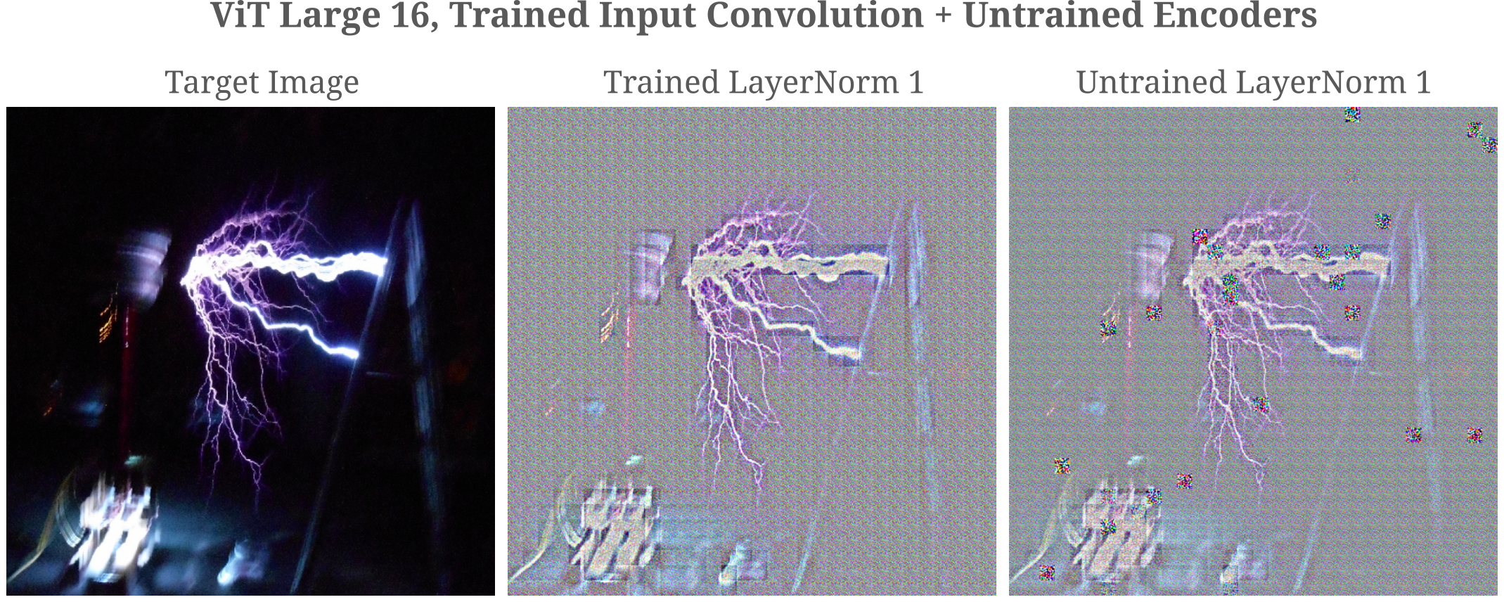
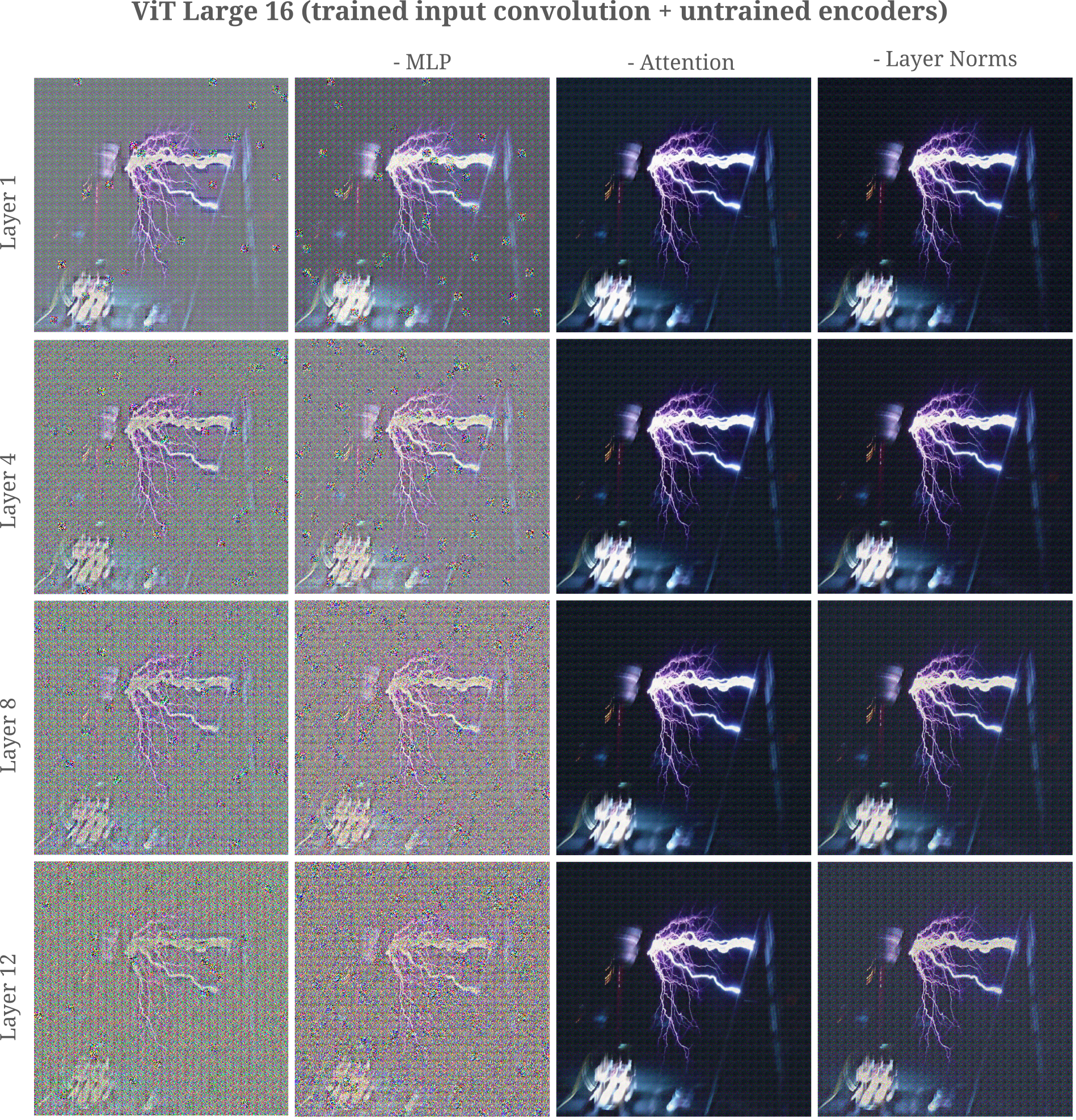
We are now going to focus on ViT Large 16, where the ‘trained’ modules are pretrained on weakly supervised datasets before being trained on ImageNet 1K, and images are all 3x512x512.

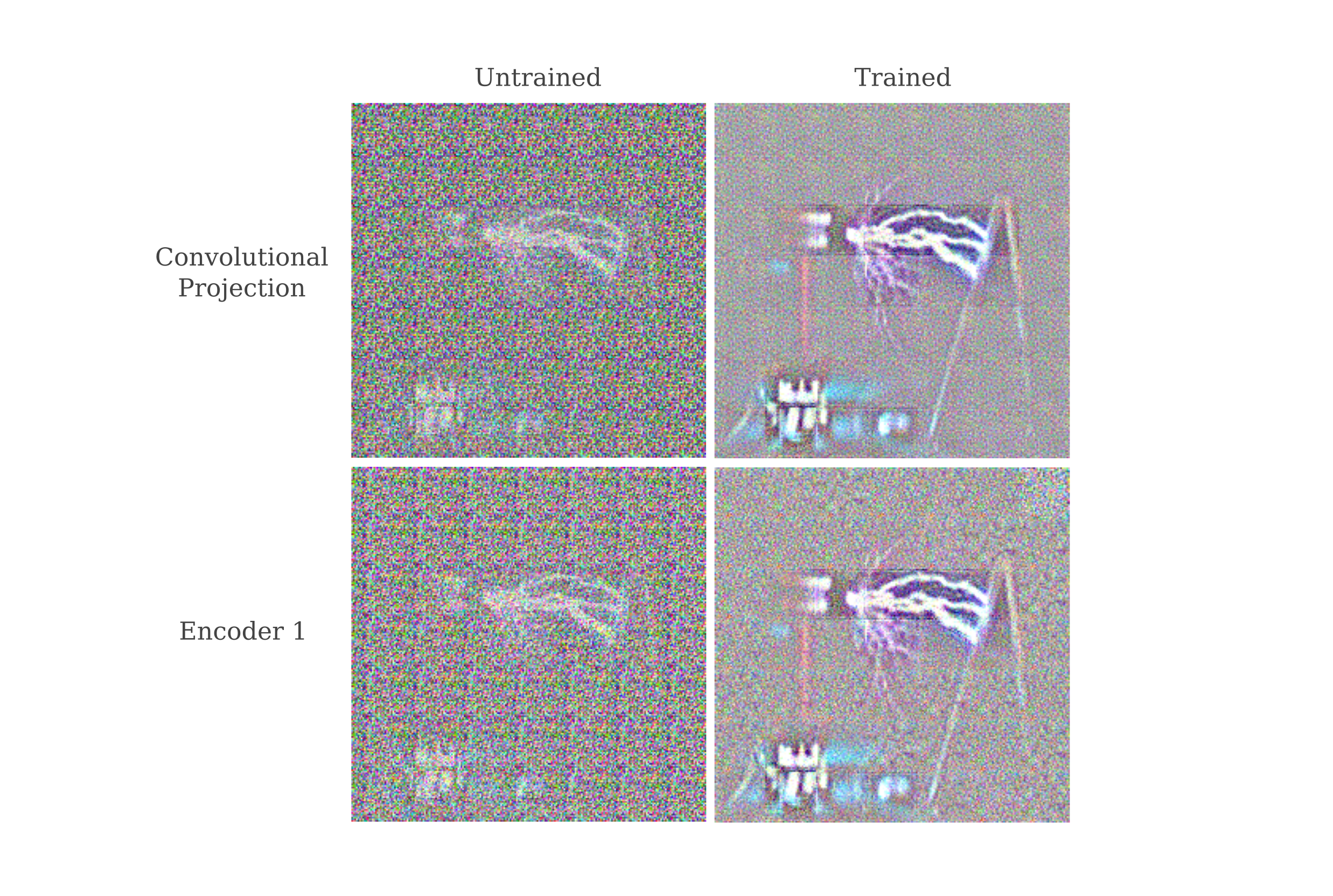
The first thing to note is that this model behaves similarly to ViT Base 32 with respect to the input convolution: applying a trained input convolution without switching to a trained first layernorm leads to patches of high-frequency signal in the input generation, which can be ameliorated by swapping to a trained layernorm.

The approach we will follow is an ablation survey: each component will be removed one after the other in order to observe which ones are required for input representation from the module output. Change are made sub-classing the EncoderBlock module of ViT and then simply removing the relevant portions.

This class is originally as follows:

class EncoderBlock(nn.Module):
    """Transformer encoder block."""
    ...
    def forward(self, input: torch.Tensor):
        torch._assert(input.dim() == 3, f"Expected (batch_size, seq_length, hidden_dim) got {input.shape}")
        x = self.ln_1(input)
        x, _ = self.self_attention(x, x, x, need_weights=False)
        x = self.dropout(x)
        x = x + input

        y = self.ln_2(x)
        y = self.mlp(y)
        return x + y

to remove residual connections, we remove the tensor addition steps as follows:

class EncoderBlock(nn.Module):
    """Transformer encoder block."""
    ...
    def forward(self, input: torch.Tensor):
        torch._assert(input.dim() == 3, f"Expected (batch_size, seq_length, hidden_dim) got {input.shape}")
        x = self.ln_1(input)
        x, _ = self.self_attention(query=x, key=x, value=x, need_weights=False)
        x = self.dropout(x)

        y = self.ln_2(x)
        y = self.mlp(input)
        return y

Then we can replace the EncoderBlock modules in the vision transformer with our new class containing no residual connections as follows:

# 24 encoder modules per vision transformer
for i in range(24): 
    vision_transformer.encoder.layers[i] = EncoderBlock(16, 1024, 4096, 0., 0.)

Similar changes can be made to remove layer normalizations, MLPs, or self-attention modules. One problem remains, and that is how to load trained model weights into our modified transformer encoders. As we have re-built the encoders to match the architecture of the original, however, and as the residual connections contain no trainable parameters we can simply load the original trained model and replace each layer with the trained version of that layer. For example, modifying the ViT L 16 to discard residual connections before adding weighted MLP layers we have

for i in range(24): 
    vision_transformer.encoder.layers[i] = EncoderBlock(16, 1024, 4096, 0., 0.)
    
original_vision_transformer = torchvision.models.vit_l_16(weights='IMAGENET1K_SWAG_E2E_V1').to(device)
original_vision_transformer.eval()

for i in range(24):
    vision_transformer.encoder.layers[i].mlp = original_vision_transformer.encoder.layers[i].mlp

For some choice encoder representations from an untrained ViT L 16 (with a trained input convolutional stem to allow for 512x512 inputs), we have the following input representations $a_g$ given a constant $n=1000$ iterations:

For the last layer, the same number of iterations yields

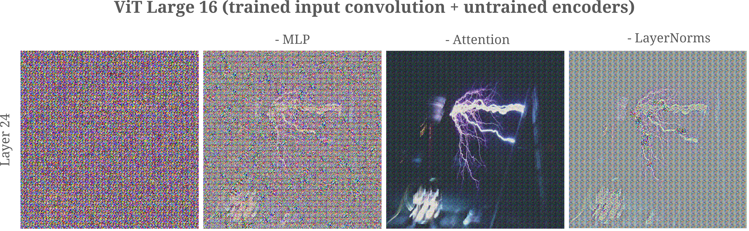
It is clear that removal of either self-attention or (both) layer normalizations in each encoder module, but not the MLPs from each encoder module is sufficient to prevent the vast majority of the decrease in representation quality with increased depth up to encodrer layer 12, whereas at the deepest layer (24) of this vision transformer we can see that removal of attention modules from each encoder (but not MLPs or LayerNorms alone) prevent most of the decline in input representation accuracy.

This is somewhat surprising given that the MLP used in the transformer encoder architecture is itself typically non-invertible: standard practice implemented in vision transformers is to have the MLP implemented as a one-hidden-layer (with input and output dimensions equal to the dimension of the self-attention hidden layer $d_{model}$) with the hidden layer three or four times as large as $d_{model}$. This MLP is identically applied to all self-attention outputs such that each embedding of the input patch after self-attention receives the same MLP. But being that the transformation from hidden to output layer of the MLP is non-invertible as there are fewer output elements than elements in theinput, there is in general not a single unique input for this layer.

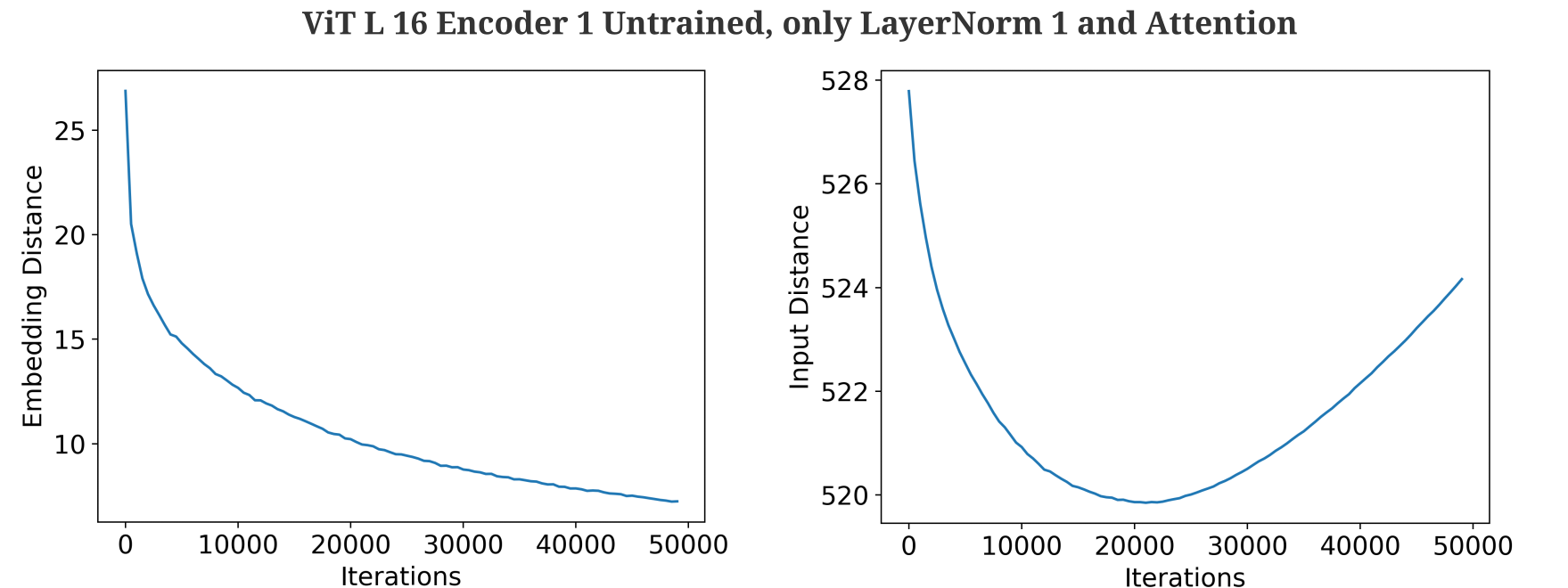
Likewise, self-attention and layernorm transformations are both non-invertible and yet removal of only one or the other appears sufficient for substantially improving input representation accuracy in early layers. From the rate of minimization of the embedding distance

\[||O(a_n, \theta) - O(a, \theta)||\]

it is clear that self-attention layers are extremely poorly conditioned: including these makes satisfying

\[||O(a_g, \theta) - O(a, \theta)|| < ||O(a', \theta) - O(a, \theta)||\]

(where $a’ = a + \mathcal{N}(a; \mu=0, \sigma=1/20$ is a slightly shifted input that is visually very similar to $a$ and $a_g$ is the final generated input representation after $n$ steps) extremely difficult for a reasonable amount of steps $n$ regardless of the update size $\epsilon$. Why this is the case will be considered below.

Removal of layer normalization transformations does not yield as much of an increase in input representation accuracy for the last layer (24) of the ViT large 16. This is because without normalization, at that depth the gradient begins to explode for certain patches: observe the high-frequency signal originating from two patches near the center of the layernormless example above. A very small gradient update rate $\epsilon$ must be used in the gradient descent procedure $a_{n+1} = a_n + \epsilon * \nabla_{a_n}O(a_n, \theta)$ to avoid sending those patch values to infinity. In turn, the finding that a vision transformer (with attention modules intact) results in exploding gradients $\nabla_{a_n}O(a_n, \theta)$ suggests that this model is poorly conditioned.

Attention does not transmit most input information

Now we will examine the effects of residual connections on input representation in the context of vision transformers. After removing all residual connections from each transformer encoder layer, we have

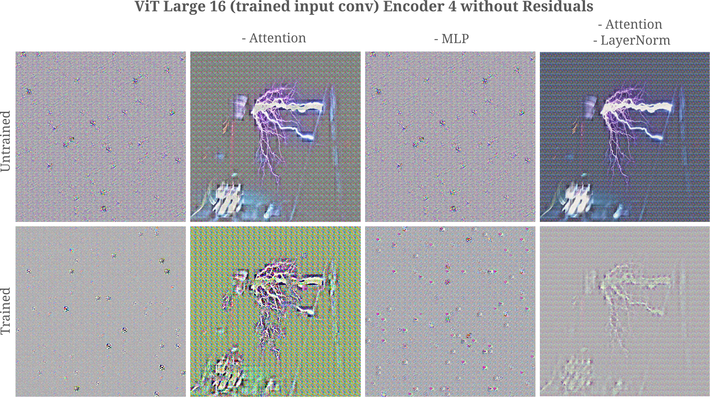
It is apparent from these results that self-attention transformations are quite incapable of transmitting most input information, which is why removing all attention modules from encoders 1 through 4 results in a recovery of the ability of the output of encoder 4 to accurately represent the input.

It may be observed that even a single self-attention layer requires an enormous number of gradient descent iterations to achieve a marginally accurate representation for a trained model, and that even this is insufficient for an untrained one. This is evidence for approximate non-invertibility, which may equivalently be viewed as poor conditioning in the forward transformation.

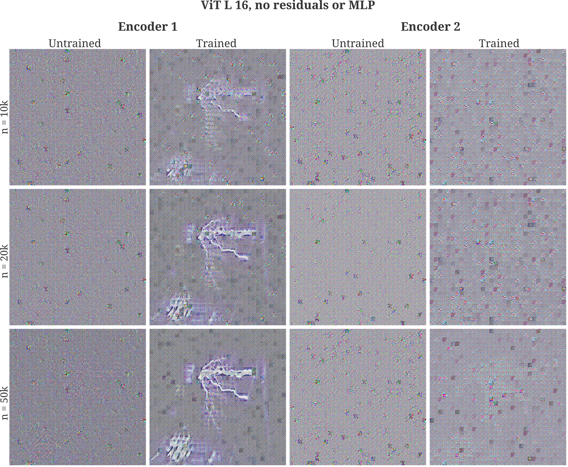
It is interesting to observe that training leads to a somewhat more informative (with respect to the input) self-attention module considering that attention layers from trained models carry very little input information with respect to fully connected layers. There may be some benefit for the transformer encoder to transmit more information during the learning procedure, but it is unclear why this is the case.

What about true non-invertibility? If our gradient descent procedure on the input is effective, then an unbounded increase in the number of iterations of gradient descent would be expected to result in an asymptotically zero distance between the target layer output $O(a, \theta)$ and the layer output of the generated input in question $O(a_g, \theta)$, or more precisely

\[a_{n+1} = a_n - g * \epsilon, \; n \to \infty \implies ||O(a, \theta) - O(a_g, \theta) ||_2 \to 0\]

If this is the case, we can easily find evidence that points to non-invertibility as a cause for the poor input representation for attention layers. For an invertible transformation $O$ such that each input $a$ yields a unique output, or for a non-invertible $O$ such that only one input $a_g$ such that $O(a_g, \theta) = O(a, \theta), a_g \neq a$ subject to the restriction that $a_g$ is sufficiently near $a$, or

\[||O(a, \theta) - O(a_g, \theta)||_2 \to 0 \implies ||a - a_g||_2 \to 0\]

On the other hand, if we find that the embedding distance heads towards the origin

\[||O(a, \theta) - O(a_g, \theta)||_2 \to 0\]

but at the input distance does not head towards the origin

\[||a - a_g||_2 \not \to 0\]

then our representation procedure cannot distinguish between the multiple inputs that may yield one output. And indeed, this is found to be the case for the representation of the tesla coil above for one encoder module with layer normalization followed by multi-head attention alone.

Thus it is apparent that self-attention layers are generally incapable of accurately representing an input due to non-invertibility as well as poor conditioning if residual connections are removed.

It is not particiularly surprising that self-attention should be non-invertible first and foremost because the transformations present in the self-attention layer (more specifically the multi-head attention layer) are together non-invertible in the general case. Recall that the first step of attention (after forming $q, k, v$ vectors) is to compute the dot product of $q, k$ vectors. The dot product, like any inner product operation, is in general non-invertible. For the case of multi-head attention where the weight matricies $W^K, W^Q, W^V$ multiplied to the input $X$ to form $q, k, v$ are non-square, this projection operation is also non-invertible. In the standard implementation of self-attention, the embedding dimension is split among the heads such that each $q, k, v$ has dimension $d=e_X/n$ where $e_X$ is the input embedding dimension and $n$ is the number of attention heads. None of these weight matricies are typically square for this reason.

With residual connections included and assuming constraints on the self-attention transformation’s Lipschitz constants (and assuming the presence of residual connections) as observed by Zha and colleages. That said, it is apparent from the experiments above that the vision transformer’s attention modules are indeed invertible to at least some degree without modification if residuals are allowed (especially if layernorms are removed).

It may be wondered how much attention layers contribute to a trained model’s input representation ability to transform the input to match the manifolds learned during training. Removing self-attention layers or MLPs from each transformer encoder, we see that there is some small highlighting of certain areas of the Tesla coil that exist in the deeper representations without attention layers but not without MLPs.

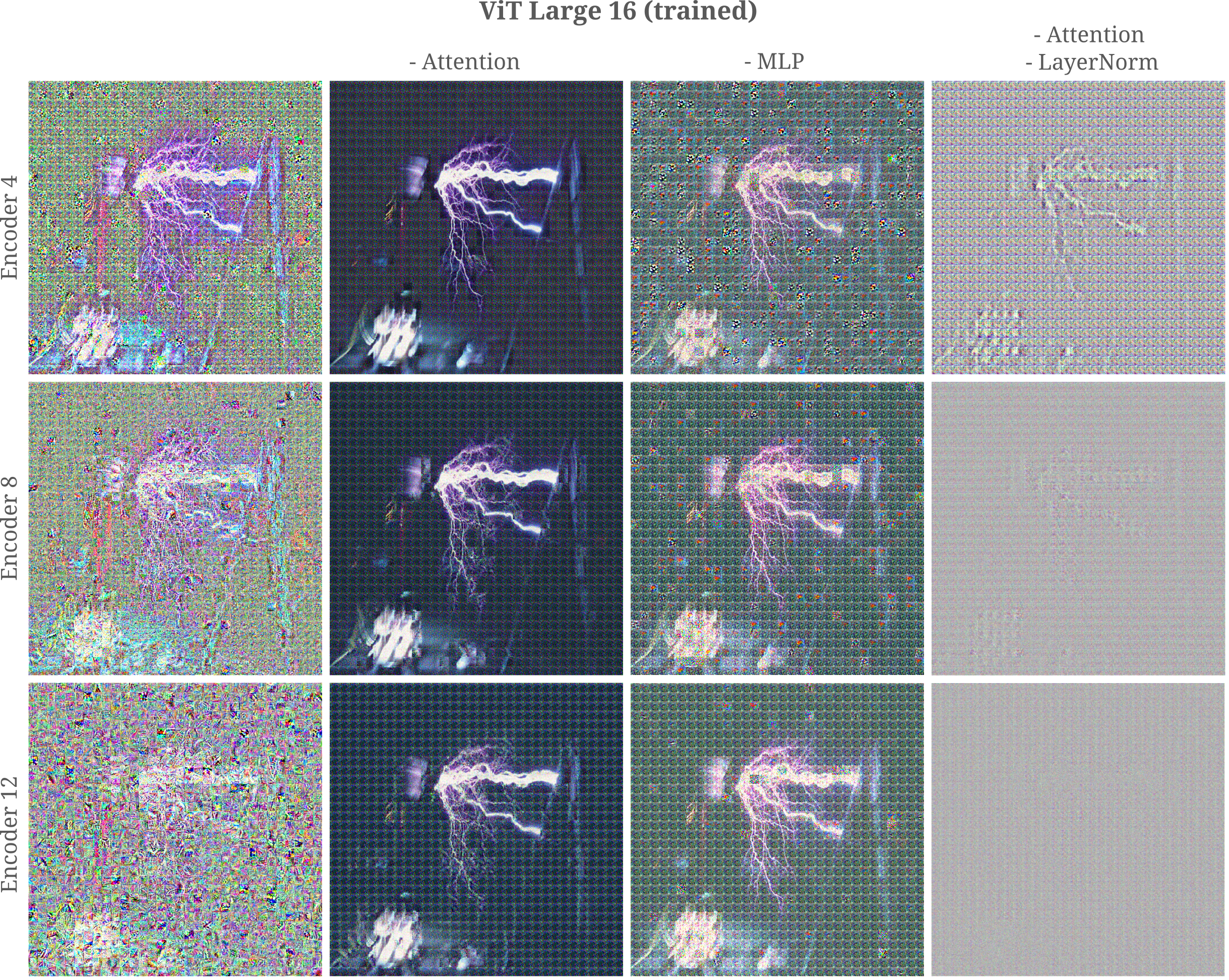
The same observations are made for an input image of a Dalmatian, which is one of the 1000 classes that the vision transformer is trained upon.

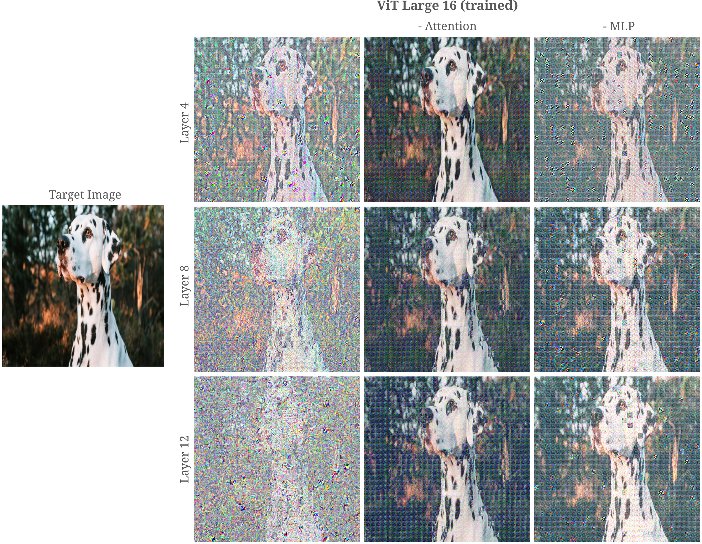
It may be appreciated that training results in a substantial increase in the ability of attention modules (in the context of ViT Large 16 without MLP layers) to represent an input, but at the same time it is apparent that each attention layer severely limits the information that passes through to the output.

As vision transformers are effective regardless of this severely limited information pass, it may be wondered whether this matters to the general goal of image classification. For the training process, there certainly is a significant effect of such information restriction: if one removes the residual connections from ViTs, the resulting model is very difficult to train and fails to learn even modest datasets such as CIFAR-10.

On the other hand, if remove residual connections from MLP-mixers (which are more or less identical to transformers except that the self-attention layer has been swapped for a transposed feed-forward one) the resulting model is not difficult to optimize, and indeed has only a limited decrease in accuracy.

Attention transformations present challenges for Gradient Descent Optimization

The process of layer representation visualization relies on gradient descent to modify an initially random input such that the layer in question cannot ‘distinguish’ between the modified input $a_g$ and some target input $a$. We have seen already that self-attention layers and layer normalization transformations result in non-uniqueness in the forward pass such that many values of $a_g$ yield one identical $O(a_g, \theta)$.

This is not necessarily a problem for the problem of classification: far from it, we typically want many inputs $a_1, a_2, …, a_n$ to map to one class output $O(a_n, \theta) = y$ for a successful classification. If the layer in question has separated the classes such that the layer’s output $O_l(a_n, \theta)$ provides a simple mapping for subsequent layers, classification is likely to be successful.

On the other hand, poor convergence of the gradient descent procedure is likely to indicate difficulty training. Suppose that it takes a very large number of iterations $n$ for the input representation gradient descent

\[a_{n+1} = a_n - \epsilon * \nabla_{a_n}J(O_l(a_n, \theta))\]

(where $J(O(a_n, \theta))$ is typically a norm of the difference between the target output and the current output, $\vert \vert O_l(a_n, \theta) - O_l(a, \theta) \vert \vert$) such that for some sufficiently small $\delta$ we have

\[|| O_l(a, \theta) - O_l(a_n, \theta) || < \delta\]

Now consider the learning procedure of stochastic gradient descent in which the model’s parameters $\theta$ are modified to minimize some objective function on the output $J(O(a, \theta))$.

\[\theta_{n+1} = \theta_n - \epsilon * \nabla_{\theta}J(O(a, \theta))\]

It can be recognized that these are closely related optimization problems. In particular, observe how the ability to minimize $\vert \vert O_l(a_n, \theta) - O_l(a, \theta) \vert \vert$ via changes in $a_n$ as $n$ increases is related to the problem of minimizing $J(O(a, \theta)$ via changes in the parameters of the first layer of our model $\theta_1$. To make things simpler, we can assume that the first layer is not fully connected by is composed of $m$ linear functions acting on $m$ input variables.

Attentionless Patch Model Representations

After the successes of vision transformers, Tolstikhin and colleagues and independently Melas-Kyriazi investigated whether or not self-attention is necessary for the efficacy of vision transformers. Somewhat surprisingly, the answer from both groups is no: replacing the attention layer with a fully connected layer leads to a minimal decline in model performance, but requires significantly less compute than the tranditional transformer model. When compute is constant, Tolstikhin and colleagues find that there is little difference or even a slight advantage to the attentionless models, and Melas-Kyriazi finds that conversely using only attention results in very poor performance.

The models investigated have the same encoder stacks present in the Vision transformers, but each encoder stack contains two fully connected layers. The first fully connected layer is applied to the features of each patch, and for example if the hidden dimension of each patch were 512 then that is the dimension of each parallel layer’s input. The second layer is applied over the patch tokens (such that the dimension of each MLP in that layer’s input is the number of tokens the model has).These models were referred to as ‘MLP-Mixers’ by the Tolstikhin group, which included this helpful graphical sumary of the architecture:

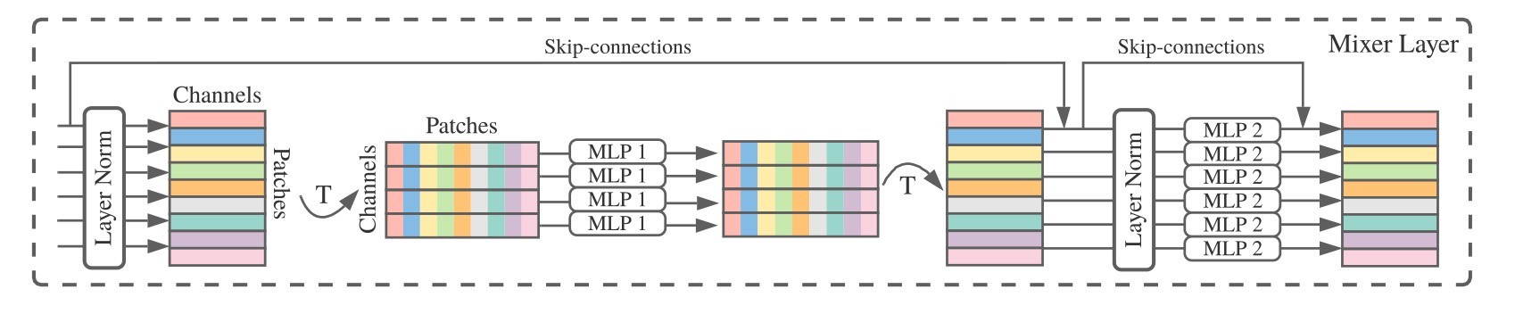
There is a notable difference between the mixer architecture and the Vision Transformer: each encoder block in the ViT places the attention layer first and follows this by the MLP layer, whereas each block in the attentionless mixer architecture has the feature MLP first and mixer second.

We investigate the ability of various layers of an untrained MLP mixer to represent an input image. We employ an architecture with a patch size of 16x16 to a 224x224x3 input image (such that there are $14*14=196$ patch tokens in all) with a hidden dimension per patch of 1024. Each layer therefore has a little over 200k elements, which should be capable of autoencoding an input of ~150k elements.

Somewhat surprisingly, this is not found to be the case: the first encoder layer for the above model is not particularly accurate at autoencoding its input, and the autencoding’s accuracy declines the deeper the layer in question. Specifying a smaller patch size of 8 does reduce the representation error.

It may be wondered why the representation of each encoder layer for the 16-sized patch model is poor, being that each transformer encoder in the model is overcomplete with respect to the input.

This poor representation is must therefore be (mostly) due to approximate non-invertibility (due to poor conditioning), and this is bourne out in practice as the distance of the model output with generated input $O(a_g, \theta)$ to the output of the target input $O(a, \theta)$ which we are attempting to minimize, ie

\[m = || O(a, \theta) - O(a_g, \theta) ||_2\]

is empirically difficult to reduce beyond a certain amount. By tinkering with the mlp encoder modules, we find that this is mostly due to the presence of layer normalization: removing this transformation (from every MLP) removes the empirical difficulty of minimizing $m$ via gradient descent on the input, and visually provides a large increase in representation clarity. For the Tolstikhin implementation, the effect of removing layer normalization is somewhat more dramatic

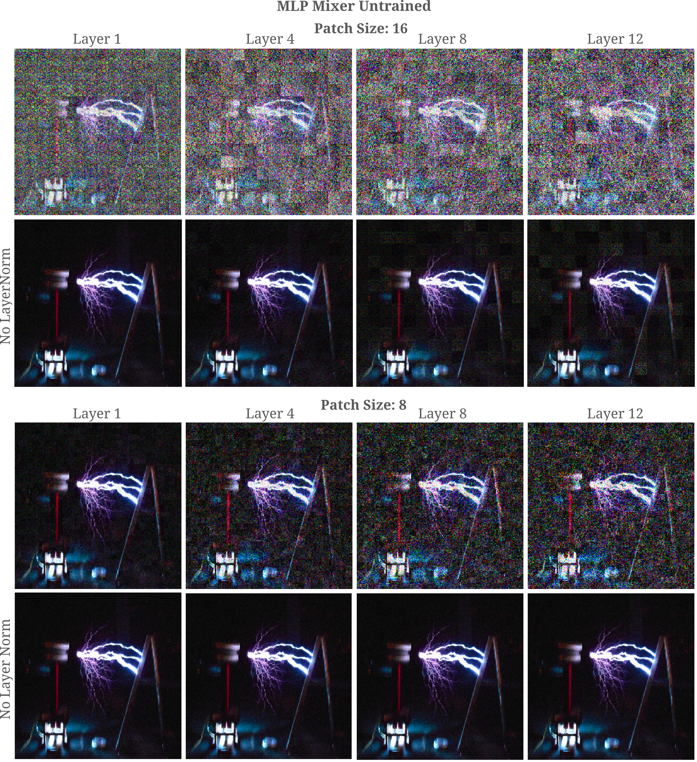
than for the Melas-Kryiazi implementation, which is shown in the following figure.

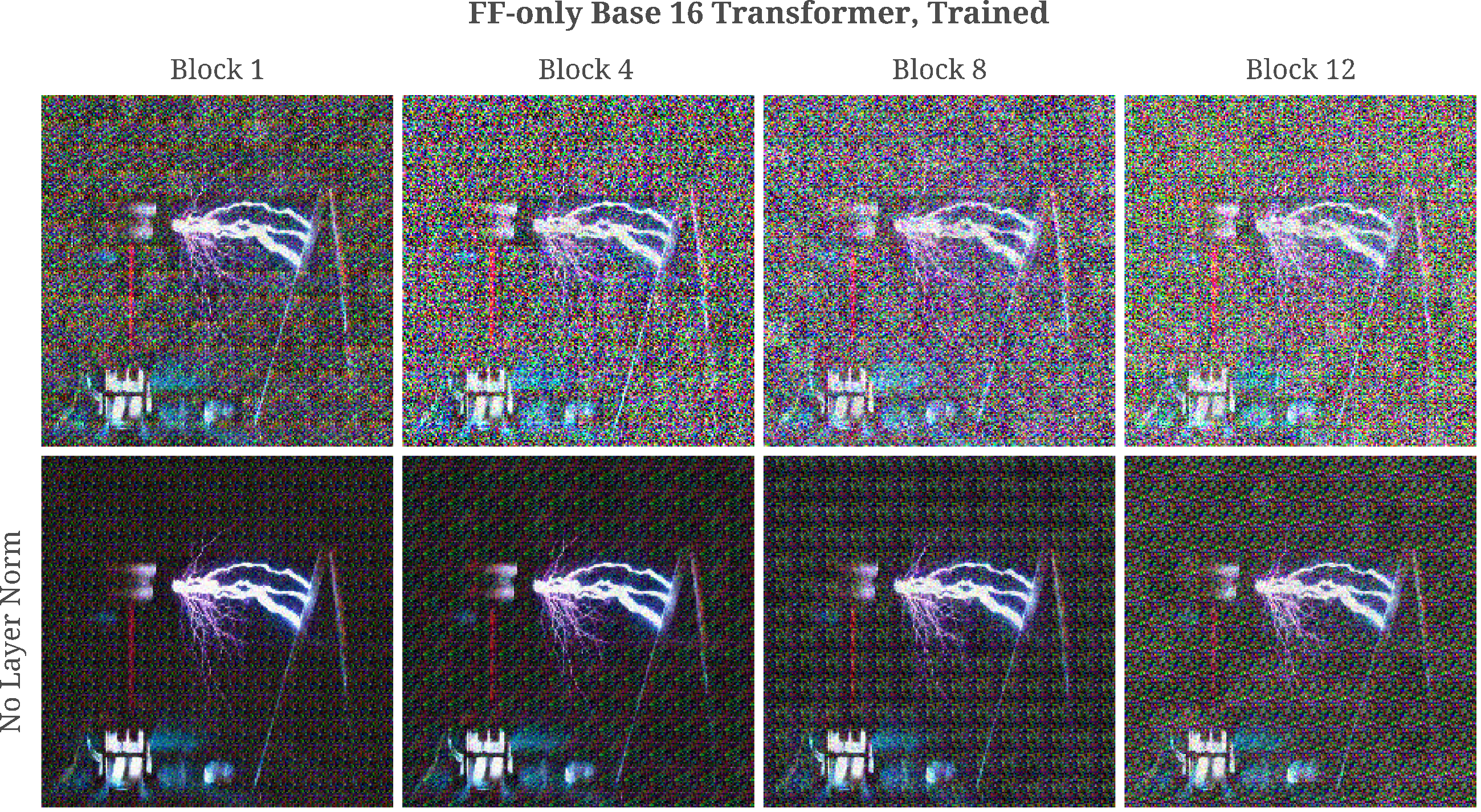
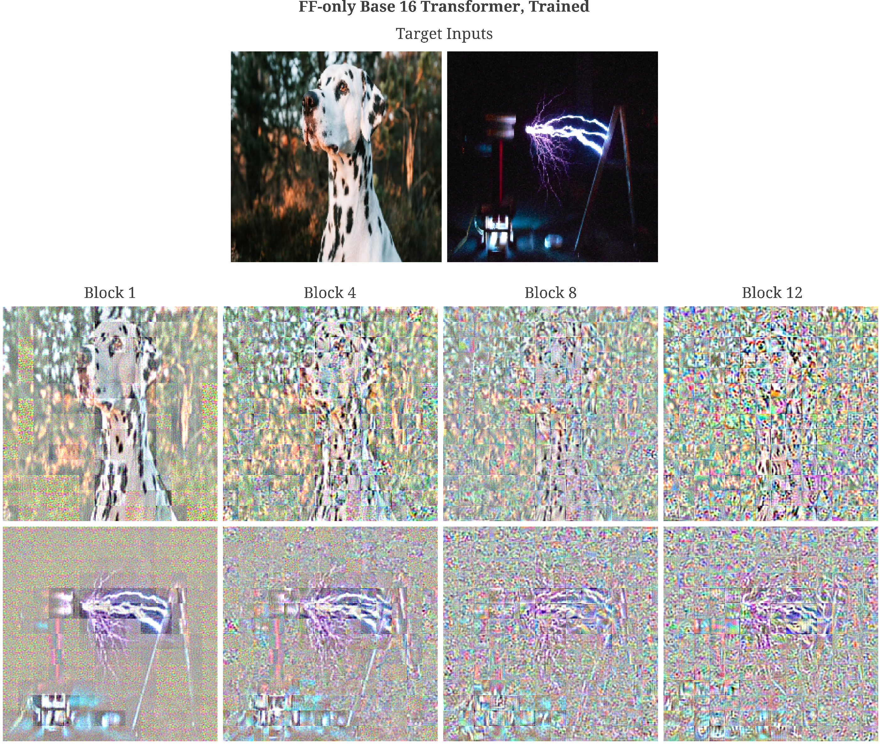
After training on ImageNet, we find that the input representations are broadly similar to those found for ViT base models, with perhaps some modest increase in clarity (ie accuracy compared to the original) in the deeper layers.

For further investigation into the features of MLP-mixers and vision transformers, see this page.