Language Model Features

Introduction

How do deep learning models make decisions? This is a fundamental question for understanding the (often very useful) outputs that these models give.

One way to address this question is to observe that most deep learning models are compositions of linear operations (with nonlinear transformations typically applied element-wise) which means that one can attempt to examine each separable component of a model in relative isolation. A particularly intuitive question one might ask is what input yields the maximum output for some hidden layer element (assuming other elements of that layer are relatively unchanged) because one may consider that input to be most ‘recognizable’ to that element.

Feature visualization studies have shown that vision models learn to identify and generate shapes via a hierarchical sequence of shape speceficity model layer: early convolutional (or transformer) layers are most activated by simple patterns or repeated shapes whereas deeper layers are most activated by specific objects or scenes. For much more information on this topic, see this page.

Background

The fundamental challenge of applying input gradient descent or ascent methods is that language model inputs are discrete rather than continuous. Therefore either some transformation must be made on the input in order to transform it into a continuous and differentiable space or else some other value must be substituted. A logical choice for this other value is to use the embedding of the inputs, as each input has a unique embedding that is continuous and differentiable.

Therefore we will observe the features present in language models by performing gradient descent on the embedding of the input.

\[e_{n + 1} = e_n - \eta \nabla_{e_n}|| c - O(e_n, \theta) ||_1\]

This procedure was considered by previously by Poerner and colleages but thought to yield generated embeddings $e_g$ that were not sufficiently similar to real word embeddings as judged by cosine distance, which is simply the cosine of the angle between angles of points in space. For vectors $a$ and $b$

\[a \cdot b = ||a ||_2 *||b||_2 \cos \phi \\ \cos \phi = \frac{a \cdot b}{|a ||_2 *||b||_2}\]

It is not clear that this is actually the case for large language models, however. This is because the value of cosine distance is extraordinarily dependent on the number of parameters of $a$ and $b$, with higher-dimensional vectors yielding smaller cosine distances. When $\cos \theta$ of the embedding of a trained Llama 7b is measured between an $e_g$ that most closely matches ‘calling’ we find that this value is much larger than the cosine distance between embeddings of ‘calling’ and ‘called’.

Secondly, elsewhere we have already seen that gradient descent on a language model embedding is capable of recovering a text input that exactly matches some given target. If $e_g$ in that case did not sufficiently resemble real inputs this procedure would have a vanishingly low probability of success.

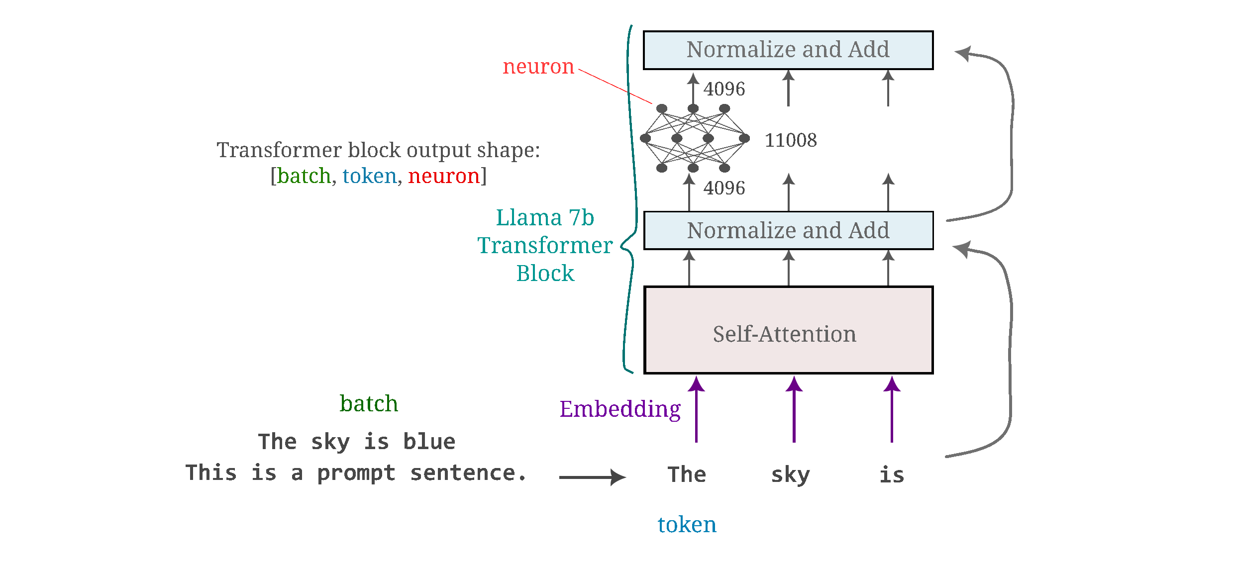
With this in mind, we can go about observing what inputs activate each neuron in various layers of language models. We will consider the outputs of transformer-based language models that are sometimes described as having a shape $[batch, \; sequence, \; feature]$. We will generate only 1-element batches, so on this page any output of shape $[:, n, m]$ is equivalent to the ouptut $[0, n, m]$ where $[:]$ indicates all of the elements of a given tensor index.

The following figure provides more detail into what exactly we are considering a ‘feature’. Each ‘feature’ is essentially a single neuron’s activation of the output of a transformer block (although it could also be assigned as the output of a transformer’s self-attention module as this is the same shape).

To find an input $a_g$ that represents each ‘feature’ of output layer $O^l$, we want to find an input $a_g$ that maximized the activation of some subset of that output layer for the model $\theta,

\[a_g = \underset{a}{\mathrm{arg \; max}} \; O^l_f(a, \theta)\]

with the reasoning that the input $a_g$ gives a large output in the feature $O^l_f$ and therefore is most emblematic of the sort of input that this feature recognizes in real inputs.

Language inputs are fundamentally discrete, and so we cannot simply perform gradient descent on the input as was done for vision models. We can, however, perform gradient descent on the embedding of an input, which is defined as the matrix multiplication of the input $a$ and an embedding weight $e$. For language models the input is typically a series of integers which is converted into a vector space embedding via a specialized weight matrix $W$. We will denote this mapping as follows:

\[e = Wa\]

and ignore the fact that $a$ cannot be multiplied directly to a weight matrix as it is not a vector for now.

We can use gradient descent on the input’s embedding where the objective function is a distance metric between a tensor of the same shape as $O^l_f$ comprised of some large constant $C$ and the output values as follows. Here we choose an $L^1$ metric on the output.

\[e_{n+1} = e_n + \eta \nabla_{e_n} (||C - O^l_f(e_n, \theta)||_1)\]

After $N$ iterations we generate $e_g$, and recover the input which maps to this embedding using the Moore-Penrose pseudoinverse

\[a_g = W^+e_g\]

where $a_g$ is a vector that can be converted to a series of tokens by taking the maximum value of each sequence element in $a_g$.

Llama features are aligned across different-sized models

Before examining which parts of a language model respond to what input, it is helpful to recall what we learned from the same question applied to vision models. For both convolutional as well as transformer -based vision models, the main finding was that shallow layers (near the input) learn features that detect simple patterns like repeated lines or checkers, whereas deeper layers learn to identify features that are much more complex (an animal’s face, for instance, or a more complicated and irregular pattern).

We focus here on the Llama family of models introduced by Touvron and colleages, which are transformer decoder-based causal language models (meaning that these models are trained to predict the next token given a series of previous tokens).

The shallowest Llama modules yield similar results as what was observed for vision models: maximizing the output of any given output neuron for all tokens (here limited to five tokens total) results in a string of identical words. For example, the feature maps of first three neurons of the first Llama transformer (7 billion parameter version) block ($O^l = 1$ if one-indexed)

\[O_f = [:, \; :, \; 0] \\ a_g = \mathtt{<unk><unk><unk><unk><unk>}\] \[O_f = [:, \; :, \; 1] \\ a_g = \mathtt{<s><s><s><s><s>}\] \[O_f = [:, \; :, \; 2] \\ a_g = \mathtt{</s></s></s></s></s>}\]

Here we will use a shorthanded notation for multiple features: $0-4$ for instance indicates features 0, 1, 2, 3, 4 (inclusive) in succession.

\[O_f = [:, \; :, \; 2000-2004] \\ \mathtt{called \; called \; called \; called \; called} \\ \mathtt{ItemItemItemItemItem} \\ \mathtt{urauraurauraura} \\ \mathtt{vecvecvecvecvec} \\ \mathtt{emeemeemeemeeme}\]

This is very similar to what is observed for vision transformers: there, the feature maps of single neurons (ie with the same shape as is observed here) in shallow layers yield simple repeated patterns in which the input corresponding to each token is more or less identical (see here.

If we observe feature maps from a single neuron at different tokens in the first module of Llama 7b, we find that the word.

\[O_f = [:, 0 - 4, 2000] \\ \mathtt{\color{red}{called}\; Iger \; Alsolass} \\ \mathtt{are \; \color{red}{called}ger \; Alsolass} \\ \mathtt{are \; I \; \color{red}{called} \; Alsolass} \\ \mathtt{are \; Iger \; \color{red}{called}lass} \\ \mathtt{are \; Iger \; Also \; \color{red}{called}} \\\]

When we combine features, somewhat unpredictable outputs are formed. For example, optimizing an input for the first four features (denoted 0:4, note that this is non-inclusive) yields

\[O_f = [:, \; :, \; 0:4] \\ a_g = </s><unk><s><s><unk>\]

and four different features combined give

\[O_f[:, \; :, \; 2000:2004] \\ a_g = \mathtt{vec \; calledura \; calledvec}\]

This is all to be expected given what was learned from features in vision models. It comes as some surprise therefore to find that different-sized Llama models have nearly identical features for the dimensions they share in common. For example, if we observe the features of the 13 billion or 30 billion parameter versions of Llama, we find exactly the same features that were present for the 7 billion parameter Llama. Note that the 13 billion Llama was trained on the same text as the 7 billion Llama, but Llama 30b was trained on more text and thus was exposed to different training data.

Transformer Block 1
=================================
Llama 13b [:, :, 2000-2004]
called called called called called
ItemItemItemItemItem
urauraurauraura
vecvecvecvecvec
emeemeemeemeeme

Llama 30b [:, :, 2000-2004]
called called called called called
ItemItemItemItemItem
urauraurauraura
vecvecvecvecvec
emeemeemeemeeme

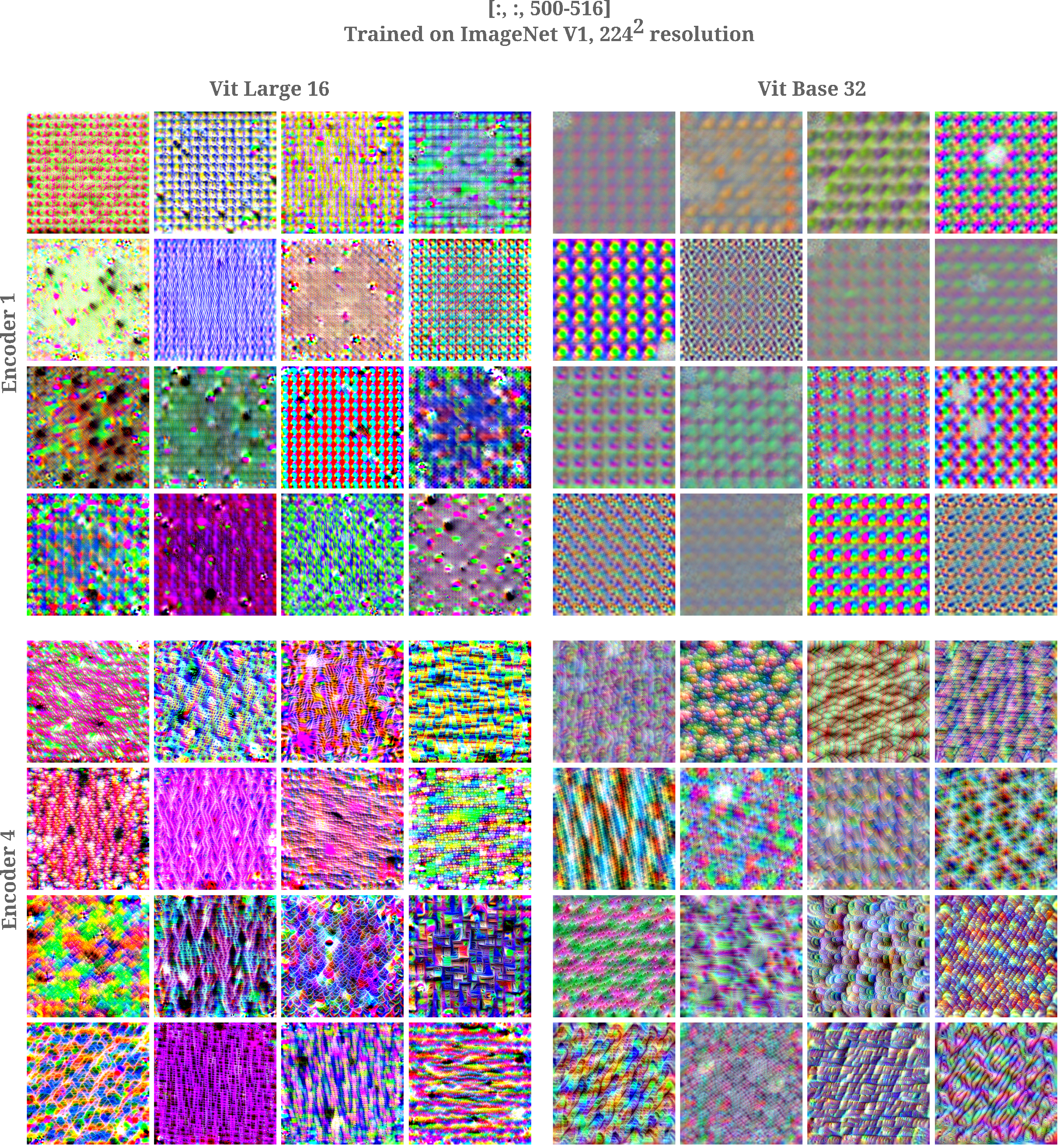
It is worth considering how different this is compared to transformer-based models that are designed for vision tasks. For vision transformers, there is little similarity between identical features for different-sized models. The following figure shows models that were trained on an identical dataset that differ by size only, with each grid location showing the feature map of a certain feature in both models.

Llama features are aligned across layers

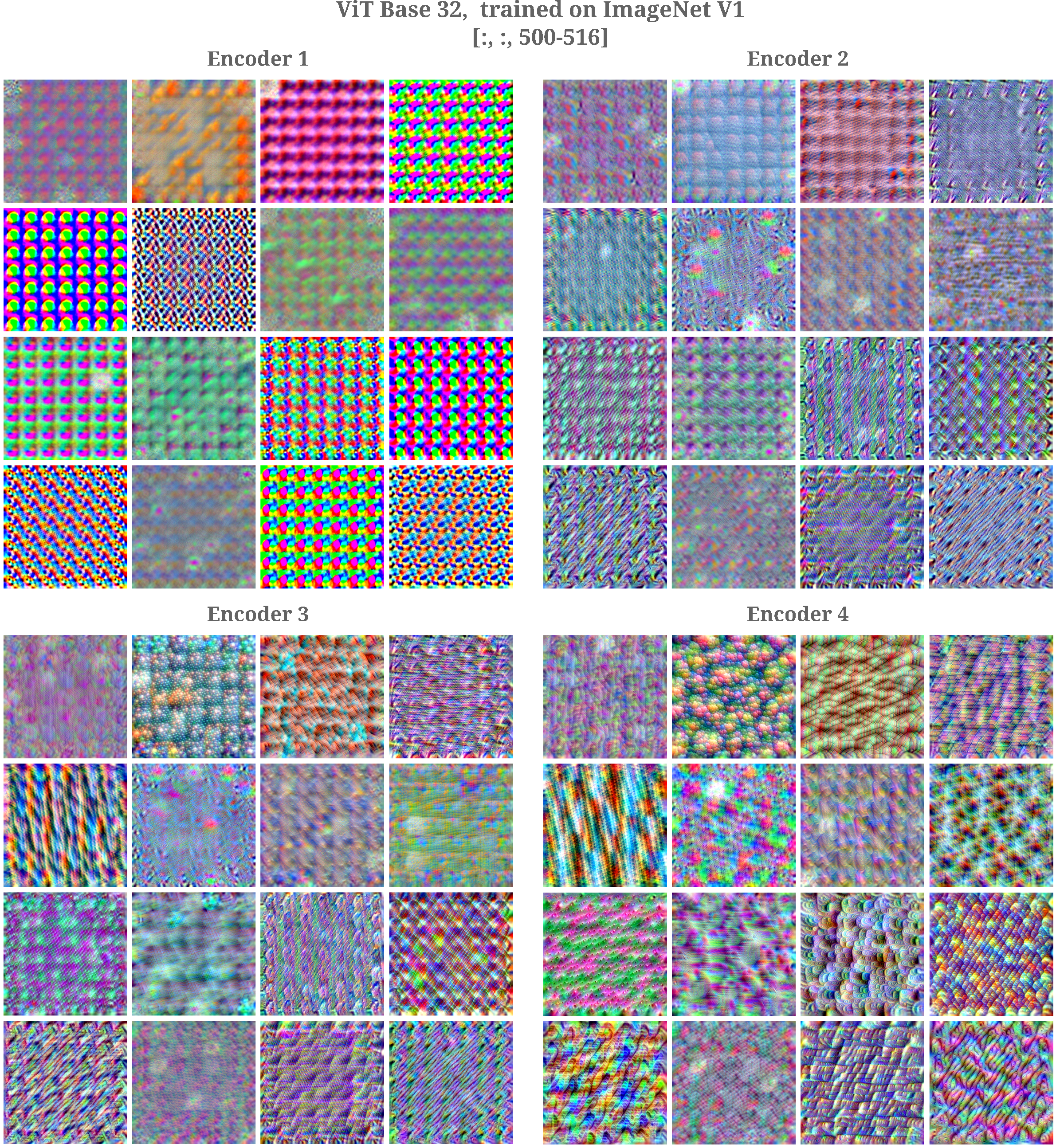
For any given vision transformer neuron, these features are typically very different between different layers. Subsequent layers may have similar features but it is far from the case that every feature in each layer is identifiable from the last layer. In the figure below, it is clear that the features of the first four transformer blocks (where forward- and back-propegation occurs through all previous blocks to the input embedding) are generally distinct.

This is in contrast to what is observed for language models, where the features of many outputs are identical. For example, given the 7 billion parameter version of Llama we have the following feature maps at the denoted layer (forward and back-propegation proceeding through all blocks prior)

Block 4
[:, :, 2000-2004]
called called called called called
ItemItemItemItemItem
urauraurauraura
vecvecvecvecvec
emeemeemeemeeme

Block 8
called called called called called
ItemItemItemItemItem
urauraurauraura
vecvecvecvecvec
emeemeemeemeeme

which is identical to what was seen at block 1. Deeper layer features are not, however, exactly identical to what is seen for shallower layers: observing the inputs corresponding to may features together at different tokens, we find that an increase in depth leads to substantially different maps for the 13 billion parameter version of Llama.

block 1
[:, 0-2, :]
ther� year раreturn
therige year раreturn
ther� year раreturn

block 4
[:, 0-2, :]
tamb would си]{da
column tamb mar marity
cal would tambIONils

block 8
[:, 0-2, :]
ports mar mar user more
endports marре user
tamb marports Elie

block 12
[:, 0-2, :]
ports mar tamb El mar
ports mar cды
tamb marportsiche mar

It may also be wondered what the features of each layer (without all preceeding layers) look like. We see the same identical input representations in most layers of Llama 13b (or Llama 7b or 30b for that matter). For example, for the 32nd transformer block of this model we see the same features as those we saw for the 1st transformer block.

O_f = [:, :, 2000-2003]
called called called called called
ItemItemItemItemItem
urauraurauraura
vecvecvecvecvec

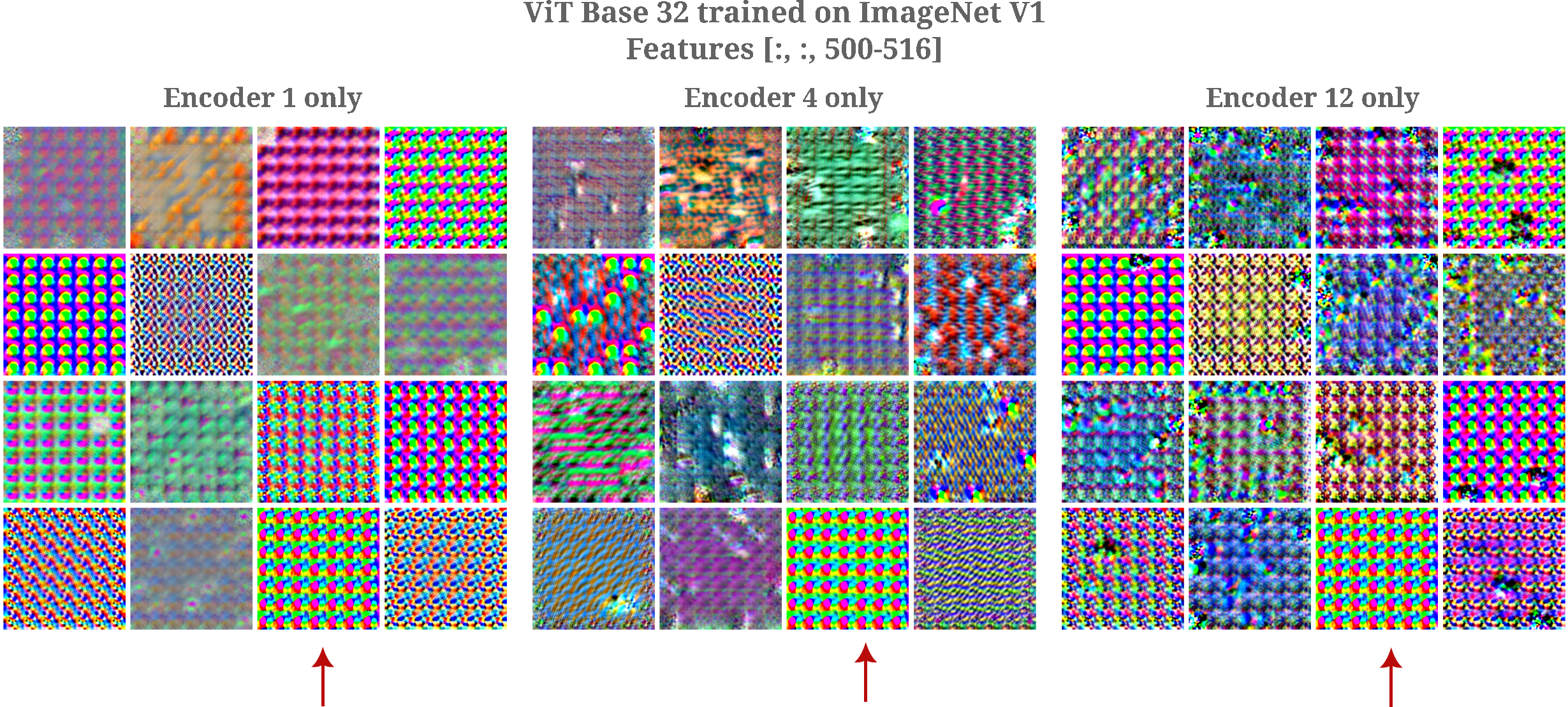
This is also not found in vision transformers: although certain features tend to be more or less identical across many transformer blocks the majority are not.

Trained Llama features closely resemble untrained ones

Even more surprising is that an untrained Llama 7b would have identical features to the trained model.

Block 1
==================================
O_f = [:, :, 0-2]
<unk><unk><unk><unk><unk>
<s><s><s><s><s>
</s></s></s></s></s>

[:, :, 2000-2004]
called called called called called
ItemItemItemItemItem
urauraurauraura
vecvecvecvecvec
emeemeemeemeeme

When a single feature is optimized at different tokens, we find that as for the trained Llama model the token corresponding to the self token

[:, 0-2, 2000]
calledremger partlass
are calleddata Alsolass
are I calledamplelass
are Idata calledlass
are Idataample called

Block 4
[:, :, 2000]
are calleddata called met
Item larItemItem met
uraFieldurauraura
vecvecvec reallypha

[:, 0-2, :]
ypearchárodyause
ci helriesiти
haromenIndoz és

Heterogeneous features in a large Llama

So far we have seen that features are remarkably well-aligned in Llama-based language models. But when we investigate the larger versions of Llama more closely, we find that

Llama 30b
Block 1
[:, :, 2000-2002]
called called called called called
ItemItemItemItemItem
urauraurauraura

Block 4
[:, :, 2000-2002]
called called called called called
ItemItemItemItemItem
urauraurauraura

Block 32 
[:, :, 2000-2002]
called planlearason current
******** doesn())ason current
ura statlearason current

We also find that features of multiple neurons are quite different when comparing Llama 30b to Llama 13b,

block 4
Llama 30b
[:, 0-2, :]
osseringering How
oss yearsering yearsoss
estooss yearsoss

Llama 13b
[:, 0-2, :]
tamb would си]{da
column tamb mar marity
cal would tambIONils

Complete Search Features

It may be wondered whether or not the feature generation method employed on this page is at all accurate, or whether the gradient descent-based generated inputs are unlike any real arrangement of tokens a model would actually observe.

Because we are working with fixed-vocabulary language models, we can go about testing this question by performing a complete search on the input: simply passing each possible input to a model and observing which input yields the largest output for a particular output neuron will suffice. We will stick with inputs of one token only, as the time necessary to compute model outputs from all possible inputs grows exponentially with input length (for GPT-2 for $n$ tokens there are $50257^n$ possible inputs).

Specifically, we want the input index $i$ that maximizes the output of our chosen output layer’s feature $O^l_f$.

\[a_i = \underset{a}{\mathrm{arg \; max}} \; O^l_f(a, \theta)\]

We begin with the smallest version of GPT-2, which contains 117m parameters. By batching inputs, we can iterate through every possible input in around two seconds on a T4 GPU. On a trained model, we have for the first four features $[:,\; :,\; 0-4]$

	[:,:, 0]	[:, :, 1]	[:, :, 2]	[:, :, 3]
Block 1	Pwr	Claud	Peb	View
Block 2	ItemTracker	watched	Peb	(@
Block 4	ItemTracker	watched	Peb	(@
Block 8	ItemTracker	watched	Peb	(@

Complete search finds different tokens than gradient descent on the input or on the embedding. For example, performing gradient descent on $\nabla_e \vert \vert O(e_n, \theta) - O(e, \theta) \vert \vert_1$ on the same output yields

for, im, G,$

or cosine distance of the angle $\phi$ between vectorized versions of the output $O(e_n, \theta)$ and the target output $o(e, \theta)$ (ie $\nabla_e \cos(\phi)$) we have

!, ", qu, $

It is notable that we come to the same conclusion as with gradient-descent based feature visualization: the features of each neuron at a given index are aligned across a range of layers. GPT-2 medium (355m parameters) we find the same $[:,\; :,\; 0-4]$

	[:,:, 0]	[:, :, 1]	[:, :, 2]	[:, :, 3]
Block 1	Ender	pmwiki	Cass	catentry
Block 4	refres	Flavoring	carbohyd	assetsadobe
Block 8	refres	Flavoring	carbohyd	assetsadobe
Block 12	refres	Flavoring	carbohyd	assetsadobe

This alignment of features across many layers is the result of training and is not present in randomly-initialized models: if we explore the features corresponding to $O_f = [:,\; :,\; 0-4]$ of an untrained 117m parameter GPT-2, we find

	[:,:, 0]	[:, :, 1]	[:, :, 2]	[:, :, 3]
Block 1	Yan	criticizing	policy	Pont
Block 4	inski	Giants	consuming	Bert
Block 8	distruptions	erie	N	Aut
Block 12	video	collection	wipe	EngineDebug

which is what one would expect if the activation of any given neuron (at a specific layer) was random with respect to the input.

Gradient descent with priors

As the complete search method becomes computationally infeasible for larger inputs, we instead use gradient descent. Ideally want there to be a match between gradient descent-based feature visualization and complete search for short inputs, but we have seen that this is not the case.

Recalling what was learned for vision model feature visualization, it is natural to wonder whether enforcing some Bayesian prior on the gradient descent process. In the context of vision models applied to images of the natural world, feature visualization commonly adds priors of positional invariance (by re-scaling the input during generation) and local smoothness (by performing Gaussian convolution).

What priors should be enforced on a language model input? So far on this page we have explored performing gradient descent on vector-space embeddings of discrete inputs (which naturally cannot be used for gradient descent without conversion to a continuous vector space of some kind). It is unclear if there are any universal priors to enforce on a language model embedding, but there is certainly a distribution-based prior one could enforce on an input that was more directly generated. This is because if we (pseudo)invert the embedding transformation $E$ (which is $E^+ = (E^TE)^{-1}E^T$ and may be thought of as the inverse of $E$ that minimizes the $L^2$ metric on the solution vector $\vert \vert a^* \vert \vert_2$ for the equation $a^* = E^+y$. With our output $y = E(a)$, this is equivalent to

\[a^* = E^+ \left( E(a) \right)\]

Typically we find that $a^*$ is approximately a one-hot vector, which signifies a vector with one entry non-zero (typically one) and all others identically zero ($[0, 0, 1, 0]$ for example). Any vector with non-identical elements may be transformed into a one-hot vector by simply assigning the value one to the maximum value of the vector and zero elsewhere. But we also want an input that may be optimized via gradient descent, and unless one were to assign a very large learning rate to the gradient this direct transformation to a one-hot vector is not useful for our purposes.

Instead we can take an idea from causal language modeling: in order to prevent a function from returning a differentiable vector that differs too much from the range of a one-hot vector. To prevent the generated input $a_g$ from diverging too much from $a’’$ we can apply a softmax transformation during every iteration of gradient descent to make

\[a_{n+1} = \mathrm{softmax\;} \left(a_n - \nabla_a ||O(a_n, \theta) - O(a, \theta)|| \right)\]

When this method is applied to the 117m parameter GPT-2, we find that the input tokens do not correspond to those found via complete search, as instead we have:

	[:, :, 0]	[:, :, 1]	[:, :, 2]	[:, :, 3]
Block 1	cris	Cola	Cass	Holt
Block 4	Geh	20439	og
Block 8	Geh	20439	expend	assetsadobe

Greedy Search Features

In light of the difficulties are presented by gradient-based feature visualization, we return to take a second look at the complete search method introduced above. We can make an observation that causal language models (which only infer the next word in a sentence, and are the type of model investigated on this page) exclusively read inputs from left to right (as long as they are trained on English and romance languages, for example, rather than languages like Hebrew). This suggests that when building an input that maximizes a model’s feature, we can build it exclusively left to right as well.

We focus on maximizing a given feature of the hidden layer’s last sequence output only (rather than maximizing the feature over all sequence elements) and iteratively build the input by adding the token yielding maximal output of this feature to the end of the input, for a pre-determined number of iterations $N$ (equaling the token number). The reason for this is that maximizing each last token only yields the maximal output if each maximal output is chosen per iteration, ie we undergo a greedy search.

To be precise, for $n \in (0, 1, …., N)$ we find $a_n$ by

\[a_n = \underset{a_n}{\mathrm{arg \; max}} \; O^l_{(f, n)}( a_n | a_{0:n-1}, \theta)\]

We can further improve the computational efficiency of this greedy approach by batching together many inputs and feeding them to the model simultaneously. This can be implemented as follows:

@torch.no_grad()
def search_maximal(n_tokens, feature, batch_size=1000):
    vocab_size = model.transformer.wte.weight.shape[0]
    maximal_tokens = []
    for t in range(n_tokens):
        activations = []
        for i in range(0, vocab_size, batch_size):
            token_batch = torch.tensor([j for j in range(i, min(i + batch_size, vocab_size))])
            token_batch = token_batch.reshape((min(batch_size, vocab_size - i), 1)).to(device)
            maximal_tensor = torch.tensor(maximal_tokens).repeat(min(batch_size, vocab_size - i), 1).to(device)
            if t > 0:
                greedy_tokens = torch.cat((maximal_tensor, token_batch), dim=1).int()
            else:
                greedy_tokens = token_batch
            output = a_model(greedy_tokens)
            activations += output[:, -1, feature].flatten()

        activations = torch.tensor(activations)
        token_int = torch.argmax(activations)
        maximal_tokens.append(token_int)

    tokens = tokenizer.decode(maximal_tokens)
    return tokens

For the 117m parameter version of GPT-2, we have the following for $N=4$

Trained GPT-2 Base
[:, :, 0-3]
Block 1 
 Pwr PwrItemTrackerItemTracker
 Claud Lara Lara Lara
 Peb Peb Peb Peb
Viewtnctnctnc

Block 4 
ItemTracker interf interfItemTracker
watched watched watched watched
Peb Peb Peb Peb
 (@"></ guiName"></

Block 8 
ItemTracker interf interf interf
watched watched watched watched
 Peb Peb Peb Peb
(@ guiName"></ guiName

Block 12 
ItemTracker interf interf interf
 hostages herpes herpes herpes
 Kenn Peb Peb Peb
(@rawdownloadcloneembedreportprintrawdownloadcloneembedreportprintrawdownloadcloneembedreportprint

Once again we observe that the alignment of features between layers is a learned phenomenon, as the untrained 117m parameter GPT-2 yields inputs with no correlation between layers for identical features (see the following figure).

Untrained GPT-2 Base
[:, :, 0-3]

Block 1
Officers ii Denis variability
onductASE Media tissue
 Comp accusationShiftShift
 separated activekef patented

Block 4
 Abortion contention variability variability
 one 185 (" Ic
 coin Foss multiplied multiplied
 Ae archetype faded faded

Block 8
 Preferencesstrip Installation Installation
 one logosAmy sheet
coin tiles unique backstory
 active MDMA incentiv thirst

It should be noted, however, that this alignment is not quite as absolute as was observed for gradient descent-based methods or for 1-token length complete search. It is evident that GPT-2 model transformer blocks exhibit more closely aligned features than those in vision transformers, where it is usually not possible to determine features in block $n-1$ features given features from block $n$.

To see that the greedy approach using only the last sequence element’s activation is equivalent to the greedy approach using all sequence activations, we can modify the algorithm as follows:

def search_maximal(n_tokens, feature, batch_size=1000):
    ...
        output = a_model(greedy_tokens)
        focus = output[:, :, feature]
        aggregated_focus = torch.sum(focus, dim=-1)

and repeating the experiment above, we find that the same inputs are generated. This is because language model transformer blocks only observe tokens to the left of a given sequence index (ie the third transformer block sequence element observes tokens 0, 1, 2, and 3 but not 4). Therefore as only the last token is chosen, only the last transformer block sequence feature determines this token.

It is interesting to note that other models exhibit less alignment in their features after training: for example, for a trained Llama 7b we have for features [:, :, 0-3] in the first dozen transformer blocks (this model has 32 total)

Block 1
Hein Hein mang Hein
cyl szere Woj cyl
inf inf char inf
travers travers assim feb

Block 4
</s></s>
cylнциклоuvud Externe
character postgresql mysqliAppData
</s>Q</s>l

Block 8
</s></s>
cyllista Which Peru
</s></s></s></s>
</s>Q</s>Q

Block 12
</s></s>
cyl которой|чення
characterparameters\ \
</s>武²).

Observe that the first token in each block is identical for each feature, but that the following tokens are typically not the same among different blocks. For deeper layers, this is no longer the case and an arbitrary feature in a certain block is typically non-identifiable from the same feature in previous blocks.

Block 16
1!--puésugo
 dataframe Broad Mediabestanden
</s> rép оп нап
</s>武性ktiv

Block 20
</s> thor webpack winter
 Cés That roughly
 .= Repub‏
� traject traject traject

Block 24
</s>CURCURCUR
aussianclar circuit
</s> rép оп §
1) traject/

Implications of feature alignment

The finding that features are at least partially aligned, particularly between layers of one model or of similar models, is remarkable for a number of reasons. Firstly, the alignment is much stronger than what is seen for vision models, even vision transformers that mirror the decoder-only transformer models used for language modeling. Secondly, there is little theoretical basis for why different transformer modules would have such well-aligned features, particularly those that are defined on gradient-descent based feature visualization methods.

But perhaps most usefully this observation of feature alignment suggests that one can easily combine layers (ie transformer block modules or even individual linear transformation layers) from various different language models to make combination models. The reason for this is that different layers from different models are more likely to have new information than different layers from the same model, being that many models have layers with quite repetitive features, and may not contain as much new information as would be beneficial to a language tasks.

This is particularly interesting in light of the findings that large language models contain parameters that are approximately normal with a few exceptions that are large outliers among practically all layers. Compressing each layer has proven difficult without resorting to parameter quantization methods, but removing and adding entire layers without further modification has not been a well-researched route.

On the other hand, there exists the beginnings of the sort of pure model merging detailed above already (meaning where one takes layers from various models and merges them together if of the same model family and size, without any additional transformations between layers) to make a single model (sometimes called a ‘Frankenmodel’). For example the Goliath 120b model is a direct merge two Llama 70b variants, and in the hands of the author is much superiour to instruction-tuned Llama-70b when it comes to factual recall, reasoning, and problem solving tasks.