Roots of polynomial equations part I
This page is the first of a two-part series on methods to find polynomial roots. For more exploration on Newton’s method, and how it relates to Julia and Mandelbrot sets, see part II.
Introduction
Algebraic polynomials are equations of the type
\[ax^n + bx^{n-1} + cx^{n-2} + \cdots + z \tag{1} \label{eq1}\]Given any polynomial, the value or values of $x$ such that the polynomial evaluates to zero are called the roots of that equation. Such value(s) of $x$ are also called the solutions of that equation because once known the polynomial may be split into parts called factors. Or alternatively if one knows how to factor a polynomial, one can then recover its roots. By the fundamental theorem of algebra, every polynomial has at least one root and therefore \eqref{eq1} contains exactly $n$ (not necessarily distinct) roots in $\Bbb C$.
At first glance, rooting polynomials in terms of their constants seems to be an easy task. For a degree 1 polynomial (meaning that $n=1$), $y = ax + b$, setting $y$ to $0$ and solving for x yields
\[x = -b/a\]For a degree 2 polynomial $ax^2 + bx + c$, the roots
\[ax^2 + bx + c = 0\]may be expressed as
\[x^2 + (b/a)x = -c/a\]Completing the square by adding $b^2/4a^2$ to both sides,
\[ax^2 + \frac{b}{a}x + \frac{b^2}{4a^2} = \frac{b^2}{4a^2} - \frac{c}{a} \\ \tag{2} \label{eq2}\]the left-hand term is now equal to
\[\left( x + \frac{b}{2a} \right) ^2\]such that when we square root both sides of \eqref{eq2},
\[x + \frac{b}{2a} = \pm \sqrt{\frac{b^2}{4a^2} - \frac{c}{a}} \\ x = \frac{-b \pm \sqrt{b^2-4ac}}{2a}\]At this point, there is no clear indication that we cannot find a similar expression for any arbitrary polynomial, but there is some slight indication that finding the expression may be very difficult because completing the square is not a method that is necessarily applicable to higher powers.
For degree 3 polynomials of the form $ay^3 + by^2 + cy + d$, a change of variables achieved by substituting $y = x - \frac{b}{3a}$ gives $x^3 + ax + b$, and a real root of this resulting equation may be found as follows
\[x = \sqrt[3]{\frac{-b}{2} + \sqrt D} + \sqrt[3]{\frac{-b}{2} - \sqrt D} \\ D = \frac{a^3}{3^3} + \frac{b^2}{2^2}\]Similarly, for polynomials of degree 4 a closed form root expressions in terms of $a, b, c …$ may be found even though the expression becomes quite long.
It is somewhat surprising then that for a general polynomial of degree 5 or larger, there is no closed equation (with addition, subtraction, multiplication, nth roots, and division) that allows for the finding of all roots. This is the Abel-Ruffini theorem, and exactly which polynomials can and cannot be rooted is explored in Galois theory.
The finding that there is no closed expression for any general finite polynomial implies the somewhat counterintuitive idea that some polynomials of degree 5 or more cannot be broken apart into factors (of any smaller degree) using a finite number of the fundamental operations of arithmetic, even though the polynomial itself is defined using these operations. The inability to find a system’s constituent parts given the whole system itself is a general feature of nonlinearity, and is witnessed on many pages of this site.
Newton’s method for estimating roots of polynomial equations
What should one do to find the roots to a polynomial, if most do not have closed form root equations? If the goal it to approximate a root, rather than express it as a combination arithmetic operations we can borrow the Newton-Raphson method from analysis. The procedure, described here, involves first guessing a point near a root, and then finding the x-intercept of the line tangent to the curve at this point. These steps are then repeated iteratively such that the x-intercept found previously becomes the x-value of the new point. This can be expressed dynamically as follows:
\[x_{n + 1} = x_n - \frac{f(x_n)}{f'(x_n)}\]After a certain number of iterations, this method usually settles on a root as long as our initial guess is reasonable.
Let’s try it out on the equation $y = x^3 - 1$, which has one real root at $x = 1$ and two complex roots
\[\frac{-1+i\sqrt{3}}{2}, \frac{-1-i\sqrt{3}}{2}\]These values are called the cube roots of unity, because they are solutions to the equation $x^3 = 1$. The complex valued roots may be found by converting $x^3-1$ to $(x-1)(x^2+x+1)$ and then applying the quadratic formula to the second term.
How does Newton’s method do for finding any of these roots? We can see by tracking each iterative root guess and looking for convergence, which is when subsequent values come closer and closer to each other until they are equivalent. Dynamically, convergence is described as a period 1 trajectory, because there is only 1 iteration of the equation (in this case Newton’s method) before the same value is reached again. The progress of root finding with Newton’s method may be tracked as follows (link to code for this page):
#! python3

def successive_approximations(x_start, iterations):
	'''
	Computes the successive approximations for the equation
	y = x^3 - 1.
	'''
	x_now = x_start
	ls = []
	for i in range(iterations):
		f_now = x_now**3 - 1
		f_prime_now = 3*x_now**2

		x_next = x_now - f_now / f_prime_now
		ls.append(x_now)
		x_now = x_next

	return ls
Let’s try with an initial guess at $x=-50$,
print (successive_approximations(-50, 20))
~~~~~~~~~~~~~~~~~~~~~~~~~~~~~~~~~~~~~~~~~~~~~~~
[-50, -33.333200000000005, -22.221833330933322, -14.813880530329783, -9.874401411977551, -6.579515604587147, -4.378643733243303, -2.9017098282008416, -1.894884560449859, -1.1704210552983418, -0.5369513549799065, 0.7981682581594858, 1.0553388026381803, 1.002851080311187, 1.0000080978680779, 1.0000000000655749, 1.0, 1.0, 1.0, 1.0]
There is convergence on the (real) root, in 17 iterations. What about if we try an initial guess closer to the root, say at $x=2$?
print (successive_approximations(2, 10))
~~~~~~~~~~~~~~~~~~~~~~~~~~~~~~~~~~~~~~~~~~~~~~~~~
[2, 1.4166666666666665, 1.1105344098423684, 1.0106367684045563, 1.0001115573039492, 1.0000000124431812, 1.0000000000000002, 1.0, 1.0, 1.0]
The method converges quickly on the root of 1. Now from this one might assume that starting from the point near $x=0$ would result in convergence in around 8 iterations as well, but
print (successive_approximations(0.000001, 20))
~~~~~~~~~~~~~~~~~~~~~~~~~~~~~~~~~~~~~~~~~~~~~~~
[1e-06, 333333333333.3333, 222222222222.2222, 148148148148.14813, 98765432098.76541, 65843621399.17694, 43895747599.451294, 29263831732.96753, 19509221155.311684, 13006147436.874454, 8670764957.916304, 5780509971.944202, 3853673314.6294684, 2569115543.0863123, 1712743695.3908749, 1141829130.2605832, 761219420.173722, 507479613.44914806, 338319742.29943204, 225546494.86628804]
a root is not found in 20 iterations! It takes 72 to find converge on a root if one starts at the origin. By observing the behavior of Newton’s method on three initial points, it is clear that simple distance away from the root does not predict how fast the method will converge. Note that the area near $x=0$ is not the only one that converges slowly on a root: $-0.7937…$ and $-1.4337…$ do as well.
Why does an initial value near 0 lead to a slow convergence using Newton’s method? Notice that the starting value was not exactly 0. Remembering that $x^3-1$ has a tangent line parallel to the x-axis at point $x=0$, and that parallel lines never meet, it is clear that Newton’s method must fail for this point because the tangent line will never meet the x-axis. Now consider why there must also be one other point that fails to converge using Newton’s method: one tangent line of $x^3-1$ intersects the origin precisely, and therefore the second iteration of Newton’s method for this point will cause the method to fail. The precise location of this first point may be found by setting $x_{n+1}$ to 0 and solving for $x_n$,
\[x_{n+1} = x_n - \frac{f(x_n)}{f'(x_n)} \\ 0 = x - \frac{x^3-1}{3x^2} \\ -\sqrt[3]{\frac 12} = x\]or equivalently, as the tangent line with slope $m = 3x^2$ must pass through both the origin $x_0, y_0$,
\[y - y_0 = m(x - x_0) \\ y - 0 = 3x^2(x - 0) \\ y = 3x^3\]subject to the condition that the pair of points $(x, y)$ exists on the line $y = x^3-1$,
\[y = 3x^3, y = x^3-1 \implies \\ 0 = 2x^3 + 1 \\ -\sqrt[3]{\frac12} = x\]Which evaluates to around $-0.7937…$. But because there is one point, there must be an infinite number of other points (not necessarily distinct) along the real line that also fail to find a root because for every initial value $v_i$ that fails with this equation, there is another $v_{i2}$ such that that $v_i$ is the second iteration of Newton’s method on $v_{i2}$ and so on. To illustrate, setting the next iteration to our value just found,
\[-\sqrt[3]{\frac12} = x - \frac{x^3-1}{3x^2} \\ 0 = 2x^3 + 3 \left( \sqrt[3]{\frac12} x^2 \right) + 1\]To find this point exactly, the formidable cubic formula is required. Evaluating this yields $x= -1.4337..$. It can be appreciated now how difficult it is to find the $n^{th}$ region counting backwards from the origin that does not converge, as each iteration must be calculated in sequence.
Now consider the equation
\[y = (x-2)(x-1)(x+3) = x^3-7x+6\]with roots at $x=-3, x=1, x=2$. Again there is more than one point on the real line where Newton’s method fails to converge quickly. We can plot the pattern such points make as follows: darker the point, the faster the convergence. Lines of color corresponding to points on the real line are used for clarity.
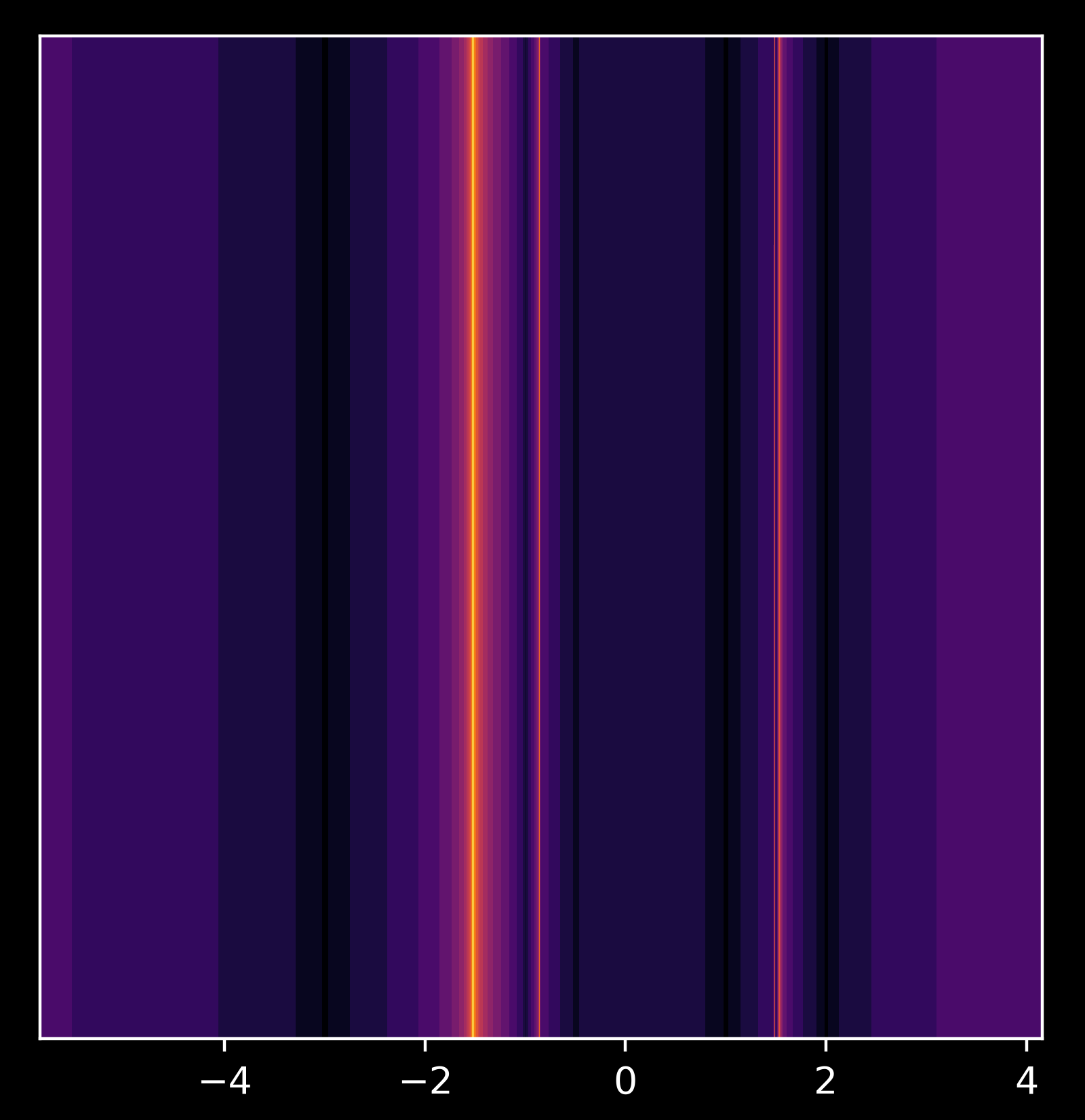
This plot seems reasonable, as the points near the roots converge quickly. Looking closer at the point $x= - 0.8410713881$,
we find a Cantor set. Not only does this polynomial exhibit many values that are slow to find a root, as was the case for $x^3 - 1$, but these non-converging points form a fractal. To see which values are in the set of non-converging points, first observe that Newton’s method will fail for points where $f’(x) = 0$, and as $f’(x) = 3x^2-7$ this evaluates to $x = \pm \sqrt{7/3}$.
We have found one non-converging value, but are there more? Yes, because any point whose next iteration of Newton’s method that lands on $\pm \sqrt{7/3}$ will also not converge. By setting $x_{n+1} = \sqrt{7/3}$ we have
\[x_{n+1} = x_{n} - \frac{f(x_{n})}{f'(x_{n})} \\ \sqrt{7/3} = x_{n} - \frac{x_{n}^3-7x_{n}+6}{3x_{n}^2-7} \\ x_{n} = −0.8625...\]which is the second line passed on the left in the video above. Setting $x_{n+1} = -0.8625$ and applying Newton’s method again and solving for $x_n$
\[-0.8625... = x_{n} - \frac{x_{n}^3-7x_{n}+6}{3x_{n}^2-7} \\ x_{n} = 1.4745...\]In other words, if $x_0 = \sqrt{7/3}$ then
\[x_{-1} = −0.8625...\\ x_{-2} = 1.4745... \\ x_{-3} = -0.8413...\\ x_{-4} = 1.47402...\]all of which are algebraic but none of which are rational.
It turns out there are an infinite number of distinct points of $x_n \; n \in \Bbb Z$, but they are contained within $[-3, 2]$ ie the region between two of the roots.
Newton’s method in the complex plane
The method used above for tracking progress made by Newton’s method can also be applied for a complex starting number, for example
print (successive_approximations(2 + 5j, 20))
~~~~~~~~~~~~~~~~~~~~~~~~~~~~~~~~~~~~~~~~~~~~~
[(2+5j), (1.325009908838684+3.3254062623860485j), (0.8644548662679195+2.199047743713538j), (0.5325816440348543+1.4253747693717602j), ... (-0.5+0.8660254037844386j), (-0.5+0.8660254037844387j)]
where Newton’s method finds the complex root
\[\frac{-1+i\sqrt{3}}{2}\]This means that the complex plane may be explored. Because Newton’s method requires differentiation and evaluation of a polynomial, I wrote a module Calculate to accomplish these tasks (which may be found here). Now a map for how long it takes for each point in the complex plane to become rooted using Newton’s method may be generated as follows:
# import third party libraries
import numpy as np
import matplotlib.pyplot as plt

from Calculate import Calculate # see above


def newton_raphson_map(equation, max_iterations, x_range, y_range, t):
	"""
	Generates a newton-raphson fractal.

	Args:
		equation: str, equation of interest
		max_iterations: int, number of iterations
		x_range: int, number of real values per output
		y_range: int, number of imaginary values per output
		t: int

	Returns:
		iterations_until_rooted: np.arr (2D) of iterations until a root is found
			at each point in y_range and x_range

	"""

	print (equation)
	y, x = np.ogrid[0.7: -0.7: y_range*1j, -1.1: 1.1: x_range*1j]
	z_array = x + y*1j

	iterations_until_rooted = max_iterations + np.zeros(z_array.shape)

	 # create a boolean gridof all 'true'
	not_already_at_root = iterations_until_rooted < 10000

	nondiff = Calculate(equation, differentiate=False)
	diffed = Calculate(equation, differentiate=True)


	for i in range(max_iterations):
		print (i)
		previous_z_array = z_array
		z = z_array
		f_now = nondiff.evaluate(z)
		f_prime_now = diffed.evaluate(z)
		z_array = z_array - f_now / f_prime_now

		# the boolean map is tested for rooted values
		found_root = (abs(z_array - previous_z_array) < 0.0000001) & not_already_at_root
		iterations_until_rooted[found_root] = i
		not_already_at_root = np.invert(found_root) & not_already_at_root

	return iterations_until_rooted
The idea here is to start with a grid of the complex plane points that we are testing (z_array), a numerical table iterations_until_rooted tracking how many iterations each point takes to find a root and a boolean table not_already_at_root corresponding to each point on the plane (set to True to start with) to keep track of which points have found a root. An small value (not 0, due to round-off error) which is 0.0000001 then compared to the difference between successive iterations of Newton’s method in order to see if the point has moved. If the point is stationary, the method has found a root and the iteration number is recorded in the iterations_until_rooted table. Note that we are only concerned with whether a root has been found, not which root has been found.
Now we can call this function to see how long it takes to find roots for $x^3 - 1$ as follows
plt.style.use('dark_background')
plt.imshow(newton_raphson_map('x^3-1', 50, 1558, 1558, 30), extent=[-5, 5, -5, 5], cmap='twilight_shifted')
plt.axis('on')
plt.show()
plt.close()
which yields
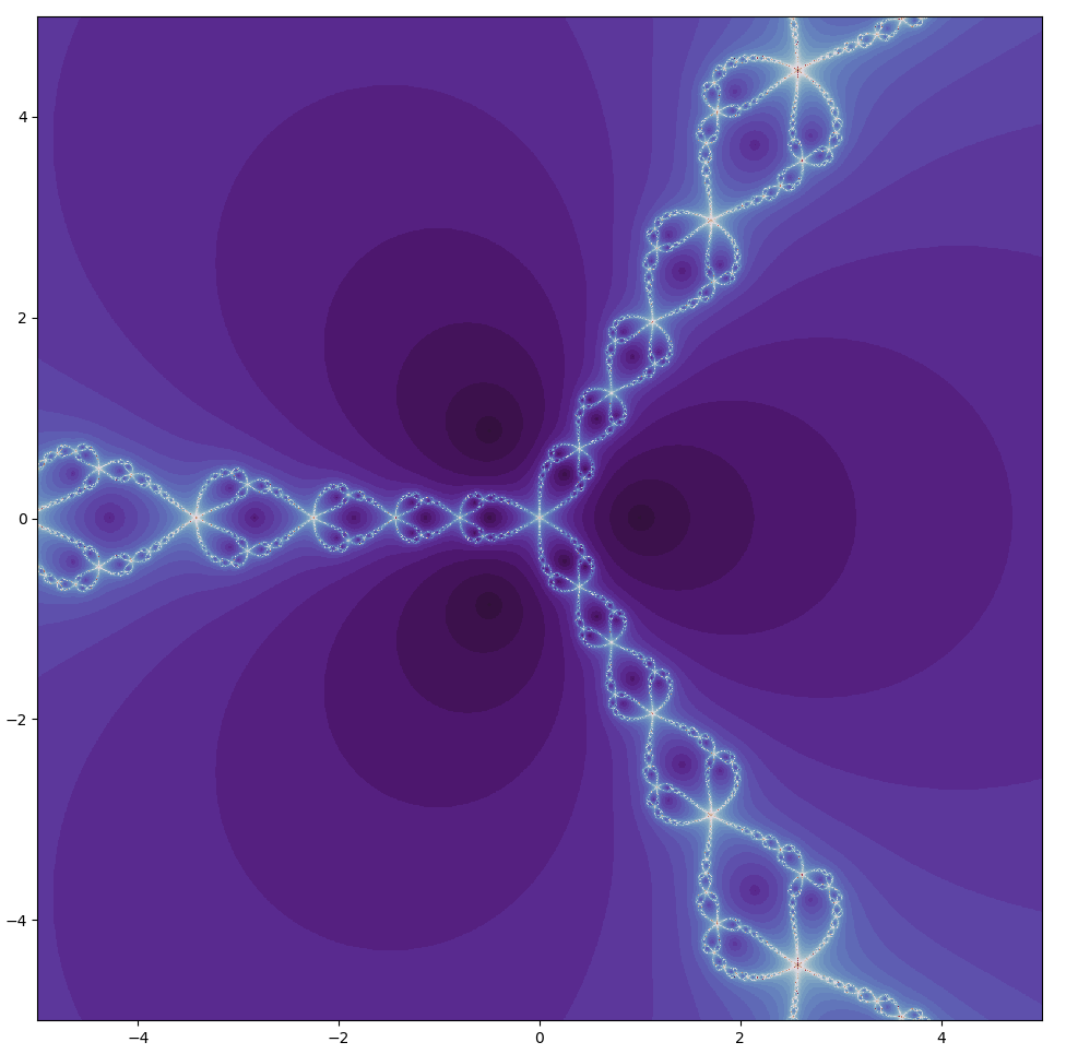
Note that for this color map, purple corresponds to fast convergence and white slow, with no convergence (within the allotted iterations) in black for emphasis. John Hubbard was the first person to observe the fractal behavior of Newton’s method in the complex plane, and the border between the set of non-diverging and diverging points may be considered to be a Julia set.
The roots for $z^3-1$ (dark circles in the plot above) may be plotted along a circle centered around the origin. This is true not just for that equation but for any root of unity or indeed any root of any complex number by De Moivre’s theorem,
\[z^n = r^n(\cos n\theta + i \sin n\theta )\]where $\theta$ is in radians of counterclockwise rotation from the positive real axis.
The above image has symmetry about the real axis (the horizontal line at the center). Is this a coincidence, or does symmetry around the real axis necessarily occur for Newton’s method? As long as the polynomial in question $a(x)$ contains only real coefficients, the roots are symmetric around the real axis because if $a + bi$ is a root, so is its conjugate $a - bi$. This is because we can assign a function $f(x)$ to map any point in the complex plane to its conjugate, meaning that $f(x): a - bi \to a + bi, \; a + bi \to a - bi$ for any $a, b \in \Bbb C$.
This function $f(x)$ is a structure-preserving map, also called a homomorphism, because
\[f(ab) = f(a)f(b) \; \forall a, b \in \Bbb C\]Furthermore because for any real number $a$, $f(a) = a$, for any polynomial with real coefficients $a(x)$, $f(a(x))$ contains the same constants and only converts $x$ to its conjugate. This does not change the root values of that function because $f(0) = 0$.
Moreover, the trajectory taken with Newton’s method may be expressed as a series of polynomials, all of which have real coefficients if $a(x)$ has real coefficients. Because there exists a homomorphism (actually isomorphism) from $a + bi$ to and from $a - bi$, the trajectories given equivalent $b$ are identical apart from an inversion about the real axis.
Incremental powers
What happens between integer polynomial powers? Here $z = z^2-1 \to z = z^5-1$, follow the link to see the change (right click the video while playing to loop)
And taking a closer look at the transition
\[z^{3.86} - 1 \to z^{3.886}-1\]As the polynomial’s largest power is incremented, large area of poorly-converging initial points appears as a light region to the left of the origin. This is the result of the appearance of a period-2 attractor whose points converge on the root along the negative real line as the polynomial approaches $z^4-1$
The images produced by searching the complex plane for points that converge quickly can be very beautiful. It is fascinating to explore the exquisite shapes that are made with relatively simple polynomials, so I made a web application to allow one to explore these images freely using Newton’s method (and other methods detailed towards the end of this page). Follow this link for the app.
A simple unrootable polynomial
Arguably the simplest polynomial that by Galois theory does not have a closed form rooted expression is
\[x^5 - x - 1\]This does not mean that finding the roots to this equation is impossible, but instead that there is no expression consisting of radicals $ \sqrt x$, addition, subtraction, multiplication, and division that represents the roots of this equation. How does one know that $x^5-x-1$ cannot be rooted? As a first step, one can find roots to an equation by attempting to factor it. Factoring here means representing a polynomial by two or more smaller polynomials, so $a(x) = b(x)c(x)$. Can the above expression be factored?
Perhaps the most direct way to check if a polynomial may be factored is to use Eisenstein’s irreducibility criterion, where a polynomial $a(x)$ defined as
\[a(x) = a_0 + a_1x + \cdots + a_nx^n\]is not reducible (not factorable) if there exists a prime number p such that p divides all $a$ except $a_n$, and $p^2$ does not divide $a_0$. Eisenstein’s criterion cannot be applied to our polynomial here because $1$ is not prime. It can be shown that Eisenstein’s criterion also applies if one substitutes $x$ for $x+a$ for any integer $a$, but this is also less than helpful.
Instead, realizing that any polynomial with rational coefficients may be factored into some constant times a new polynomial with integer coefficients, we can determine if our equation has a root in $\Bbb Q$, the rational numbers. This is because for any rational root of $a(x)$, $s/t$, in smallest terms then in the notation above $s \lvert a_0$ and $t \lvert a_n$.
It is an interesting result that any rational root field can be converted to an integer root field, which means that if our equation above has a root, it can be expressed as an integer. But the only $s/t$ which satisfies these conditions is 1, and by substituting $x=1$ it can clearly be seen that this value is not a root of $x^5-x-1$.
Therefore $x^5-x-1$ does not have any roots in $\Bbb Q$, and necessarily cannot be factored into a smaller polynomial of integer (or rational) values. But can we make a radical expression for any of these roots? Radicals are generally not elements of $\Bbb Q$, and so ruling out rational roots does not rule out the possibility that any root may be expressable as a finite number of integers and their roots.
The answer to this, too, is no: it turns out that neither can we construct all the roots for this equation with radicals. This is because the corresponding Galois group to this polynomial is $S_5$, the group of permutations of five elements. Which is to say that no finite addition of radicals can extend $\Bbb Q$ to the field of roots of our equation, and therefore no finite expression of with the terms desired may be constructed for the roots of this equation.
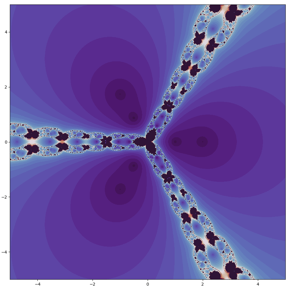
Let’s explore where roots are found with Newton’s method in the complex plane, ie for $z^5-z-1$. With a scale of $(-1.85, 2.15)$ for the real values on the horizontal axis and $(-1.86i, 2.14i)$ on the vertical (using our original color map),

Note that the roots are no longer found in a circle centered on the origin, as the equation cannot be expressed as a root of any one complex number. Looking at the roots more closely, there is one real and four complex roots: this is expected, as complex roots always come in pairs of a number and its conjugate.
Unlike the case for $z^3-1$, an entire region fails to converge on a root, rather than individual points. Now there are certainly points analagous to that observed above (for $z^3-1$) in which the tangent line is parallel to the x-axis: these exist at
\[f'(x) = 0 \\ 5x^4 - 1 = 0 \\ x = \pm \sqrt[4]{1/5} \approx \pm 0.6689...\]which corresponds to the point in the center of the 5 radial spokes to the right of the largest area of no convergence. But these do not explain the appearance of large areas of no convergence themselves.
Newton’s method yields self-similar fractals, which can be clearly observed by increasing scale. For example, zooming in on the point $0.154047 + 0.135678i$,
Newton’s map rotations
So far we have been considering polynomials with only real-valued constants and powers, or in other words polynomials $a_0x^{b_0} + a_1x^{b_1} + \cdots$ where $a_n, b_n \in \Bbb R$. This is not by necessity, and just as $x$ can be extended to the complex plane so can a polynomial itself be extended. Programs to accomplish this may be found here (use the non-optimized versions for complex-valued polynomials, as the optimized programs do not currently support complex-valued polynomials). Skip to the next section to observe what happens upon incrementing a complex power.
There is one particular transformation that is especially striking which can be accomplished by extending a polynomial’s constants and powers into the complex plane. Using the identity $e^{\pi i} + 1 = 0$, we can rotate the function in the complex plane about the origin in a radius of $1/4$ as follows:
...
for i in range(max_iterations):
		previous_z_array = z_array
		z = z_array
		f_now = z**5 - z - 1 + np.exp(3.1415j * (t/300))/4
		f_prime_now = 5*z**4 - 1
		z_array = z_array - f_now / f_prime_now
We can also perform a different rotation as follows:
...
for i in range(max_iterations):
		previous_z_array = z_array
		z = z_array
		f_now = (np.exp(3.1415j * (t/450000))/4) * z**5 - z * np.exp(3.1415j * (t/450000))/4 - 1 + np.exp(3.1415j * (t/450000))/4
		f_prime_now = 5 * (np.exp(3.1415j * (t/450000))/4)*z**4 - np.exp(3.1415j * (t/450000))/4
		z_array = z_array - f_now / f_prime_now
the cover photo for this page found here is at t=46, and at t=205 (0.00023 of a full rotation) yields

Follow the link for a video of this rotation:
Note that these are the first maps that are not symmetric about the real axis. This is because the polynomial used to iterate Newton’s method no longer has only real-valued coefficients, but instead imaginary values are introduced to accomplish the rotation. Now with $f(x)$ that transforms conjugates $a + bi, a - bi$ into one another, the coefficients are no longer unchanged and there is not an isomorphism that exists between regions of the complex plane.
Secant method
There are other methods besides that of Newton for finding roots of an equation. Some are closely related to Newton’s method, for example see the secant method in which is analagous to a non-analytic version of Newton’s method, in which two initial guesses then converge on a root.
There are two initial guesses, $x_0$ and $x_1$, which are then used to guess a third point
\[x_{n+1} = x_n - f(x_n) \frac{x_n - x_{n-1}}{f(x_n) - f(x_{n-1})}\]And so on until the next guess is the same as the current one, meaning that a root has been found. This is algebraically equivalent to Newton’s method if the derivative is treated as a discrete quantity, ie
\[f'(x) = \frac{f(x_n) - f(x_{n-1})}{x_n - x_{n-1}}\]Because there are two initial points rather than one, there is more variety in behavior for any one guess. To simplify things, here the first guess is half the distance to the origin from the second, and the second guess ($x_1$) is the one that is plotted in the complex plane. This can be accomplished as follows:
def secant_method(equation, max_iterations, x_range, y_range, t):
	"""
	Returns an array of the number of iterations until a root is found
	using the Secant method in the complex plane.

	Args:
		equation: str, polynomial of interest
		max_iterations: int of iterations
		x_range: int, number of real values per output
		y_range: int, number of imaginary values per output
		t: int

	Returns:
		iterations_until_together: np.arr[int] (2D)

	"""

	# top left to bottom right
	y, x = np.ogrid[1: -1: y_range*1j, -1: 1: x_range*1j]
	z_array = x + y*1j
	iterations_until_rooted = max_iterations + np.zeros(z_array.shape)

	 # create a boolean table of all 'true'
	not_already_at_root = iterations_until_rooted < 10000
	zeros = np.zeros(z_array.shape)

	# set the initial guess to half the distance to the origin from the second guess
	z_0 = (z_array - zeros)/2

	# initialize calculate object
	nondiff = Calculate(equation, differentiate=False)

	for i in range(max_iterations):
		previous_z_array = z_array
		z = z_array
		f_previous = nondiff.evaluate(z_0)
		f_now = nondiff.evaluate(z)
		z_array = z - f_now * (z - z_0)/(f_now - f_previous)

		# the boolean map is tested for rooted values
		found_root = (abs(z_array - previous_z_array) < 0.0000001) & not_already_at_root
		iterations_until_rooted[found_root] = i
		not_already_at_root = np.invert(found_root) & not_already_at_root

		# set previous array to current values
		z_0 = z

	return iterations_until_rooted
For $z^3-1$,
Remembering that black denotes locations that do not converge within the maximum interations (here 50), it is clear that there are more points that fail to find a root using this method compared to Newton’s, which is expected given that the convergence rate is slower than for Newton’s.
Rotated at a radius of $1/8$, $z^5-z-1$ yields
And incrementing from $z^5-z-1$ to $z^6-z-1$ we have
Halley’s method
Edmond Halley (of Halley’s comet fame) introduced the following algorithm to find roots for polynomial equations:
\[x_{n+1} = x_n - \frac{2f(x_n)f'(x_n)}{2(f'(x_n))^2-f(x_n)f''(x_n)} \;\]The general rate of convergence for this method is cubic rather than quadratic as for Newton’s method. This method can be implemented using Calculate as follows:
def halley_method(equation, max_iterations, x_range, y_range, t):
	"""
	Returns an array of the number of iterations until a root is found
	using Halley's method in the complex plane.

	Args:
		equation: str, polynomial of interest
		max_iterations: int of iterations
		x_range: int, number of real values per output
		y_range: int, number of imaginary values per output
		t: int

	Returns:
		iterations_until_together: np.arr[int] (2D)

	"""

	# top left to bottom right
	y, x = np.ogrid[1: -1: y_range*1j, -1: 1: x_range*1j]
	z_array = x + y*1j

	iterations_until_rooted = max_iterations + np.zeros(z_array.shape)

	# create a boolean table of all 'true'
	not_already_at_root = iterations_until_rooted < 10000

	# initialize calculate object
	nondiff = Calculate(equation, differentiate=False)
	diffed = Calculate(equation, differentiate=True)

	# second derivative calculation
	diff_string = diffed.to_string()
	double_diffed = Calculate(diff_string, differentiate=True)

	for i in range(max_iterations):
		previous_z_array = z_array
		z = z_array

		f_now = nondiff.evaluate(z)
		f_prime_now = diffed.evaluate(z) # first derivative evaluation

		f_double_prime_now = double_diffed.evaluate(z) # second derivative evaluation

		z_array = z - (2*f_now * f_prime_now / (2*(f_prime_now)**2 - f_now * f_double_prime_now))

		# test the boolean map for rooted values
		found_root = (abs(z_array - previous_z_array) < 0.000000001) & not_already_at_root
		iterations_until_rooted[found_root] = i
		not_already_at_root = np.invert(found_root) & not_already_at_root

	return iterations_until_rooted
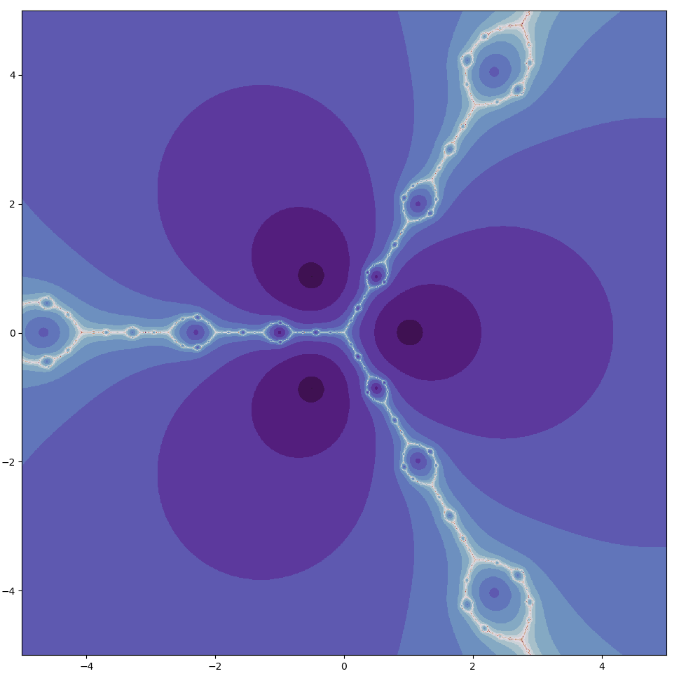
For $z^3-1$ the pattern in the complex plane of areas of slow convergence is similar but not identical to that observed for Newton’s method (see above)
For larger polynomials, areas of slow convergence are exhibited. For $z^{13}-z-1$,

and incrementing $z^{13}-z-1$ to $z^{14}-z-1$,
And similar shapes to that found for Newton’s method are also present. For $z^{9.067}-z-1$,

and incrementing $z^7-z-1$ to $z^8-z-1$,