Julia sets
A Julia (named after G. Julia) set is the boundary of the sets of unbounded and bounded iterates of the family of functions
\[f_a(x) = x^2 + a \tag{1} \label{eq1}\]where $a$ is fixed and $x_0$ varies about the complex plane $x + yi$. Different values of $a$ lead to different Julia sets, and together this family of functions $f_a(x) \forall a \in \Bbb C$ are the Julia sets.
This means that any number in the complex plane is in a Julia set if it borders another number $u$ such that iterations of \eqref{eq1} are unbounded
$f^k_a(u) \to \infty \; \mathbf {as} \; k \to \infty$
as well as a number $b$ where iterations of \eqref{eq1} are bounded
$f^k_a(c) \not\to \infty \; \mathbf {as} \; k \to \infty$
If we restrict ourselves to the real line, such that $a$ and $x$ are elements of $\Bbb R$, iterations of \eqref{eq1} have a number of interesting features. Some values of $a$ form Cantor sets (fractal dusts), which may be expected as \eqref{eq1} is a nonlinear equation similar in form to the logistic and Henon maps (see here).
Plotting Julia sets with Python
What happens when we allow $a$ and iterates of \eqref{eq1} to range over the complex plane? Let’s find out! To start with, import the indespensable libraries numpy and matplotlib
#! python3
import numpy as np
import matplotlib.pyplot as plt
and then define a function to find the values of a Julia set for a certain value of $a$, with a docstring specifying the inputs and outputs of the function. To view a Julia set, we want an array corresponding to the complex plane with values that border diverging and non-diverging values specially denoted. One way to do this is to count the number of iterations of \eqref{eq1} any given point in the complex plane takes to start heading towards infinity, and if after a sufficiently large number of iterations the point is still bounded then we can assume that the value will not diverge in the future.
To make an array of complex numbers, the class in numpy is especially helpful. We can specify the range of the x (real) and y (imaginary) planes using ogrid (special thanks to the numpy tutorial here for this idea), remembering that imaginary values are specified with j in python. The array corresponding to the complex plane section is stored as z_array, and the value of $a$ is specified (the programs presented here are designed with a value of $ \lvert a \rvert < 2 $ in mind, but can be modified for larger $a$s). This will allow us to keep track of the values of subsequent iterations of \eqref{eq1} for each point $z$ in the complex plane.
Also essential is initialization of the array corresponding to the number of iterations until divergence, which will eventually form our picture of the Julia set.
def julia_set(h_range, w_range, max_iterations):
	''' A function to determine the values of the Julia set. Takes
	an array size specified by h_range and w_range, in pixels, along
	with the number of maximum iterations to try.  Returns an array with
	the number of the last bounded iteration at each array value.
	'''
	# top left to bottom right
	y, x = np.ogrid[1.4: -1.4: h_range*1j, -1.4: 1.4: w_range*1j]
	z_array = x + y*1j
  	a = -0.744 + 0.148j
	iterations_till_divergence = max_iterations + np.zeros(z_array.shape)
To find the number of iterations until divergence of each point in our array of complex numbers, we can simply loop through the array z_array such that each point in the array is
	for h in range(h_range):
		for w in range(w_range):
It can be shown that values where $\lvert a \rvert > 2$ and $\lvert z \rvert > \lvert a \rvert$, future iterations of \eqref{eq1} inevitably head towards positive or negative infinity.
This makes it simple to find the number of iterations i until divergence: all we have to do is to keep iterating \eqref{eq1} until either the resulting value has a magnitude greater than 2 (as $z$ is complex, we can calculate its magnitude by multiplying $z$ by its conjugate $z^* $ and seeing if this number is greater than $2^2 = 4$. If so, then we know the number of iterations taken until divergence and we assign this number to the ‘iterations_till_divergence’ array a the correct index.
			z = z_array[h][w]
			for i in range(max_iterations):
				z = z**2 + a
				if z * np.conj(z) > 4:
					iterations_till_divergence[h][w] = i
					break

	return iterations_till_divergence
This will give us an iteration number for each point in z_array. What if \eqref{eq1} does not diverge for any given value? The final array iterations_till_divergence is initialized with the maximum number of iterations everywhere, such that if this value is not replaced then it remains after the loops, which signifies that the maximum number of iterations performed was not enough to cause the value to diverge. Outside all these loops, we return the array of iterations taken.
Now we can plot the iterations_till_divergence array! It is a list of lists of numbers between 0 and ‘max_iterations’, so we can assign it to a color map (see here for an explanation of matplotlib color maps). Remembering that the Julia set is the border between bounded and unbounded iterates of \eqref{eq1}, a cyclical colormap emphasizing intermediate values (ie points that do not diverge quickly but do eventually diverge) is useful.
plt.imshow(julia_set(500, 500, 70), cmap='twilight_shifted')
plt.axis('off')
plt.show()
plt.close()
Now we can plot the image!
The resolution settings (determined by h_range and w_range) are not very high in the image above because this program is very slow: it sequentially calculates each individual point in the complex array. The image above took nearly 10 minutes to make!
Luckily we can speed things up substantially by calculating many points simultaneously (well not really truly simultaneously, but using an optimized c array we can pretend that the calculations are happening a the same time) with numpy. The idea is to apply \eqref{eq1} to every value of z_array, and make a boolean array corresponding to the elements of z_array that have diverged at each iteration. The complex number array setup is the same as above, but we initialize another array not_already_diverged that is the same size as the iterations_till_divergence array but is boolean, with True everywhere as well as diverged_in_past, which is all False to begin with.
import numpy as np
import matplotlib.pyplot as plt

def julia_set(h_range, w_range, max_iterations):
	''' A function to determine the values of the Julia set. Takes
	an array size specified by h_range and w_range, in pixels, along
	with the number of maximum iterations to try.  Returns an array with
	the number of the last bounded iteration at each array value.
	'''
	# top left to bottom right
	y, x = np.ogrid[1.4: -1.4: h_range*1j, -1.4: 1.4: w_range*1j]
	z_array = x + y*1j
	a = -0.744 + 0.148j
	iterations_until_divergence = max_iterations + np.zeros(z_array.shape)

	# create array of all True
	not_already_diverged = iterations_until_divergence < 10000

	# creat array of all False
	diverged_in_past = iterations_until_divergence > 10000
Instead of examining each element of z_array individually, we can use a single loop to iterate \eqref{eq1} as follows:
	for i in range(max_iterations):
		z_array = z_array**2 + a
In this loop, we can check if any element of z_array has diverged,
$|z| > 2, z(z^* ) > 2^2 = 4$
and make a boolean array, diverging is made, which contains a True for each position in z_array that is diverging at that iteration. To prevent values from diverging more than once (as the z_array is reset to 0 for diverging elements), we make another boolean array diverging_now by taking all elements of positions that are diverging but have not already diverged (denoted by boolean values in the not_already_diverged array). Values of iterations_till_divergence that are diverging are assigned to the iteration i.
		z_size_array = z_array * np.conj(z_array)
		diverging = z_size_array > 4

		diverging_now = diverging & not_already_diverged
		iterations_till_divergence[diverging_now] = i

		not_already_diverged = np.invert(diverging_now) & not_already_diverged
In order to prevent overflow due to values heading towards infinity, values that are diverging or have diverged in the past are set to 0. It is necessary to reset values upon each iteration because for some Julia sets the value $0 + 0i$ also diverges.
		# prevent overflow (values headed towards infinity) for diverging locations
		diverged_in_past = diverged_in_past | diverging_now
		z_array[diverged_in_past] = 0

	return iterations_till_divergence
Finally the array of the number of iterations at each position is returned and an image is made
plt.imshow(julia_set(2000, 2000, 70), cmap='twilight_shifted')
plt.axis('off')
plt.show()
plt.close()
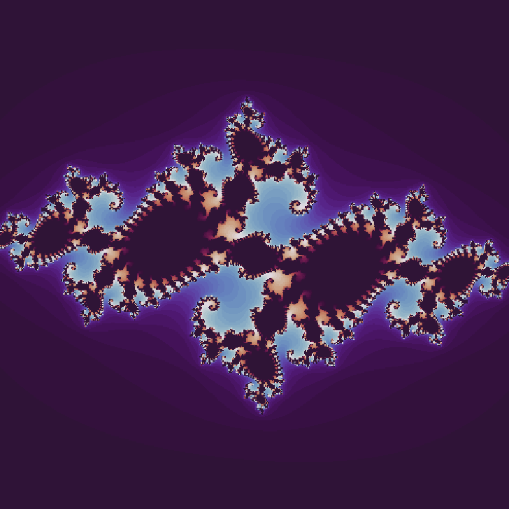
which yields for $a = -0.744 + 0.148i$:
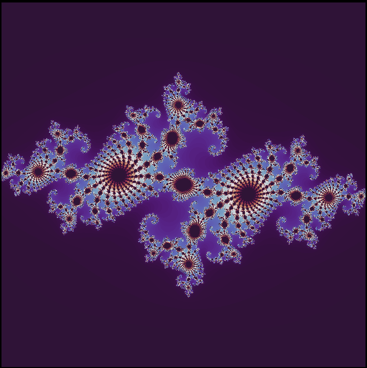
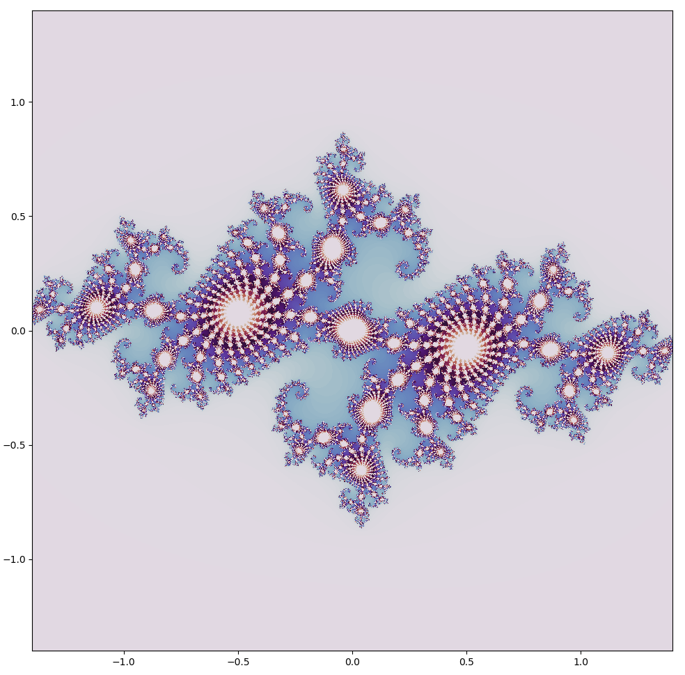
This is much faster: it takes less than a second for my computer to make the low-resolution image that previously took nearly ten minutes! Using cmap='twilight', and scaling the image by using the kwarg extent.
plt.imshow(julia_set(2000, 2000, 200), cmap='twilight_shifted', extent=[-1.4, 1.4, -1.4, 1.4])
plt.axis('on')
plt.show()
plt.close()
There are a multitute of interesting Julia sets, each one defined by a different $a$ value. We can make a video of the changes as we increment from $a=-0.29609091 + 0.62491i \to a = -0.20509091 + 0.71591i$ (how to do this is shown below) at the same scale as shown above.
There are many beautiful Julia sets that one can make! To make your own, follow this link for a web application that generates Julia sets given user input.
Julia sets are fractals
As Gaston Julia found long ago, these sets bounded but are nearly all of infinite length. Nowadays we call them fractals because they have characteristics of multiple dimensions: like 1-dimensional lines they don’t seem to have width, but like 2-dimensional surfaces they have infinite length in a finite area. Fractals are defined by having a counting dimension (Hausdorff, box, self-similarity etc) greater then their topological dimension, and nearly all fractals have fractional dimension (3/2, 0.616 etc).
To put it in another way, fractals stay irregular over different size scales. They can be spectacularly self-similar (where small pieces are geometrically similar to the whole) like many Julia sets and the Mandelbrot set, but most are not (see this excellent video by 3B1B on the definition of a fractal here. The fractals formed by the Clifford attractor and pendulum maps are not self-similar in the strictest sense.
How can a bounded line possibly have infinite length? If we zoom in on a point on the set, we can see why this is: the set stays irregular at arbitrary scale. Let’s make a video of the Julia set zoom! Videos are composed of sequences of images that replace each other rapidly (usually around 30 times per second) in order to create an approximation of motion. So to make a zooming-in video, we just need to iterate over the Julia set function defined above many times, decreasing the scale as we go!
The first thing to do is to pick a point in the complex plane to focus on, and to decide how fast the zoom should be. For an zoom that does not appear to slow down or speed up, an exponential function must be used. As magnifying an image by a power of two provides a clear image of what to think about, let’s use exponents with base 2. Say one wanted to increase scale by a factor of two over one second, with 30 individual images being shown in that second. Then each frame should be scaled by a factor of $ \frac{1}{2 ^{1/30}}$, and the way I chose to do this is by multiplying the exponent $1/30$ by the frame number t. I prefer a 4x zoom each second, so the exponent used is $t/15$.
If the scale is mostly symmetrical (nearly equal x and y ranges), that is all for the magnification process! Next we need to decide which point to increase in scale. For the Julia set defined by $a = -0.29609091 + 0.62491i$, let’s look at $x = -0.6583867 - 0.041100001i$.
def julia_set(h_range, w_range, max_iterations, t):
	# top left to bottom right grid
	y, x = np.ogrid[1.4/(2**(t/15)) + 0.041100001: -1.4 / (2**(t/15)) + 0.041100001:h_range*1j, \
			-1.4/(2**(t/15)) -0.6583867: 1.4/(2**(t/15)) -0.6583867:w_range*1j]
The julia_set() function needs to be called for every time step t, and one way to do this is to put it in a loop and save each image that results, with the intention of compiling the images later into a movie. I prefer to do this rather than compile images into a movie without seeing them first. The following code yields all 300 images being added to whatever directory the .py file running is held in, with the name of the image being the image’s sequence number.
An important step here is to increase the max_iterations argument for julia_set() with each increase in scale! If this is not done, no increased resolution will occur beyond a certain point even if we increase the scale of the image of interest. To see why this is, consider what the max_iterations value for the true Julia set is: it is infinite! If a value diverges after any number of iterations, then we consider it to diverge. But at large scale, there may not be a significatn change upon increase in max_iterations (although this turns out to not be the case for this particular Julia set, see below), so to save time we can simply start with a smaller max_iterations and increase as we go, taking more and more time per image. The true Julia set is uncomputable: it would take an infinite number of iterations to determine which $x + yi$ values diverge for all $z \in \Bbb C$, and this would take infinite time.
for t in range(300):
	plt.imshow(julia_set(2000, 2000, 50 + t*3, t), cmap='twilight')
	plt.axis('off')
	plt.savefig('{}.png'.format(t), dpi = 300)
	plt.close()
Note that keyword arguments vmin and vmax may be supplied to plt.imshow, for example by changing the second line to plt.imshow(julia_set(2000, 2000, 50 + t*3, t), vmin=1, vmax=50+t*3, cmap='twilight'). These signify the minimum and maximum range for the color map, and are not strictly necessary to make a video but prevent pyplot from initializing a new automatically defined color range for each image. This auto-scaled range is unstable, leading to consecutive images having different colors for the same numerical values which appears as flashes in the background of the video. This becomes more important for videos of polynomial root finding algorithms, among other things.
Now we have all the images ready for assembly into a movie! For my file system, the images have to be renamed in order to be in order upon assembly. To see if this is the case in your file system, have the folder containing the images listed.
(base) bbadger@bbadger:~/Desktop/julia_zoom1$ ls
My list was out of order (because some names were one digit and some 3 digits long), so I wrote a quick script to correct this.
# renames files with a name that is easily indexed for future iteration
import os

path = '/home/bbadger/Desktop/file_name_here'

files = os.listdir(path)

for index, file in enumerate(files):
	name = ''
	for i in file:
		if i != '.':
			name += i
		else:
			break

	if len(name) == 2:
		os.rename(os.path.join(path, file), os.path.join(path, ''.join(['0', str(name), '.png'])))
	elif len(name) == 1:
		os.rename(os.path.join(path, file), os.path.join(path, ''.join(['00', str(name), '.png'])))
Now that the images are in order, we can assemble them into a movie! This can be done many ways but I find ffmpeg to be very fast and stable. Here we specify a mp4 video to be made with 30 frames per second, from in order matching *.png (read ‘something’.png) and the resulting .mp4 file name is specified.
(base) bbadger@bbadger:~/Desktop/julia_zoom1$ ffmpeg -f image2 -r 30 -pattern_type glob -i '*.png' julia_zoom.mp4
which yields
The bounded line stays irregular as we zoom in (with an increased max_iterations value), and if this irregularity continues ad infinitum then any two points on this set are infinitely far from each other.
Slow divergence in a Julia set
The appearance of more diverged area (ie the purple ‘river’) in the zoom above suggests that this particular Julia set ($a = -0.29609091 + 0.62491i$) contains values that eventually diverge, but do so very slowly. Which values are these? To see this, let’s see what happens when we go from 10 to 2500 maximum iterations:
There is more and more area that diverges with an increasing number of maximum iterations. What appears to be a solid area of no divergence at a small number of maximum iterations is revealed to be a mosaic of unconnected points, of area 0.
Discontinuous transition from linear to nonlinear complex maps
Take the familiar example where $a = -0.744 + 0.148i$, but now let’s see what happens when we move from
\[f(x) = x^1 + a \to \\ f(x) = x^4 + a \tag{2}\]
We can learn a few things from these maps. The first is that non-differentiable regions (angular places) of the set experience a transition from a finite to an infinite number. This means that the maps go from mostly smooth with a few sharp angles to being entirely composed of sharp bends and twists, which is a transition from differentiability most places to nowhere-differentiability.
Another thing we can learn is that there are abrupt transitions between sets with connected areas and disconnected dusts. This is explored more fully in the Mandelbrot set, but just from these videos we can see that such changes are extremely unpredictable.