Masked Mixer Language Models
This work is continued in another blog post located here: Part II.
For the findings on both pages written in more detail and structure as an academic paper, see this paper.
Background
The training of the most effective language models today (3/2024) requires enormous computational resources: a whopping 1720320 hours of 80GB nvidia A100 compute time was required to train the 70 billion parameter version of Llama 2.
This prohibitive amount of compute power required is mostly down to the very large effective size of the models that are currently trained, rather the training dataset itself: most LLMs are trained on between 1 and 5 trillion tokens of text, but this is not actually that much information when one considers that each token is typically expressed as bytecode (ie one byte) and therefore the training dataset is a few terabytes, substantially smaller than the image datasets required to train smaller diffusion models.
Current state-of-the-art transformer models are very large indeed (>100 billion parameters) but with transformers there is another wrinkle: the key, query, and value projection weights form gradients for all of a training input’s sequence. This means that a 7 billion parameter Llama model will actually require much more space than the 7 billion params * 2 bytes per param in fp16, or 14 gibabytes one might think (if training in 16 bit precision, ignoring extra memory incurred by optimizers for the moment), and thus has an ‘effective’ parameter size much larger than the model’s actual size during inference. Together this means that it takes hundreds of gigabytes of vRAM to train a model on a small context window and with a small batch size, even though the same model may require only 14 gigabytes of memory during inference. This extra memory is due to the necessity of storing gradients on and values of attention projection weight matricies during training, making the space complexity for $n$ sequence elements $O(n^3)$ compared to the $O(n^2$) space required during inference where these values may be cached.
This begs the question: are all these parameters necessary? It is clear that transformer-based models do indeed become substantially more effective with an increase in the number of parameters they contain, but if we were not restricted to one particular architecture is it possible that we could design a model with far fewer parameters for language modeling?
By one estimate the billions of parameters are far more than would be necessary to model the English language. First consider language generation at the level of sentence completion, where the task is to simply finish a sentence. It has been claimed that there are somewhere around $m = 10^{570}$ possible English sentences as an upper bound. Without knowing how to model these sentences, we can view them as unique points in an arbitrarily high-dimension space. This being the case, we can apply a result from the concentration of measure phenomenon to greatly simplify this space.
We will make use of the Johnson-Lindenstrauss lemma, with the result that the same $m$ points may be represented with arbitrary precision in a space that is on the order of $8 \log m = 8 \ln 10^{570} \approx 1312 $ dimensional. More precisely, this lemma states that for some small $\epsilon > 0$ for set $X$ of $m$ points in $\Bbb R^N$, for
\[n > 8\ln (m) / \epsilon^2\]there is a (linear) representation map $f: \Bbb R^N \to \Bbb R^n$ where for all $u, v \in X$ the following is true:
\[(1 - \epsilon) ||u - v||^2 \leq ||f(u) - f(v)||^2 \leq (1 + \epsilon)||u - v ||^2\]Alternatively, language models today are universally trained to predict every ‘next’ token in a concatenated sequence of tokens. This means that for a training dataset of $n$ tokens, the model is trained to predict $n$ points (ignoring exactly how the sequences are concatenated and trained upon concatenation) in some presumably very high-dimensional space. The largest dataset any open-source model has been trained on is 15 trillion tokens (for llama-3), and in this case we can represent this dataset arbitrarily well in a space of approximately $8 \ln (15 \times 10^{12}) \approx 8 * 30 = 240$ dimensional. Of course, the goal of language models is to generalize to larger datasets and thus we would hope the model would accurately predict the next tokens of a much larger dataset. But even supposing that this 15 trillion token dataset is only one millionth of the size of this generalized dataset, one would still only require a space of $8 \ln (15 \times 10^{18}) \approx 8 * 44 = 352$ dimensions.
How does this relate to the number of parameters necessary in a model? Assuming that the training algorithm is sufficiently powerful (which is not at all a safe assumption, more on this later) the number of parameters in a model could correspond to one of two things: either the number of parameters in a model is equivalent to the dimensionality of the model with respect to the points it can approximate, or else the model’s ‘width’ or hidden layer dimension is equivalent to the model’s dimensionality. Because the vector space of successive layers of practically every modern deep learning model are dependent (activations in layer $n+1$ depend on layer $n$ and perhaps layer $n-1$ etc.) and dimensionality is defined on linear independence, it seems more likely that a model’s dimensionality best corresponds with its hidden layer dimension. If this is true then a model of no more than around 1300 hidden layer nodes should be capable of completing any English language sentence, or a model with a width of 350 can accurately predict a next token for a massive dataset. If these hidden widths were used for standard transformer model architectures, the resulting models would are around 100 million (350 hidden width) and 995 million (1300 hidden width) parameters.
It cannot necessarily be assumed that a model with that number of parameters is actually trainable, however: it could be that training requires a large model that must then be converted into a small model. This is the approach used when performing pruning, where parameters are dropped depending on their importance for some output. Alternatively, instead of removing parameters one could reduce the memory required to store each parameters: this is the approach of quantization methods, which are perhaps the most effective methods currently available for shrinking the effective size of a model. The observation that weight quantization rather than pruning is the most effective method for reducing a transformer model’s effective size suggests that this particular architecture may indeed require nearly all the trained parameters in order to function effectively, although whether this is the case or not remains an open questions.
Here we take the approach of investigating new architectures and training new models, rather than attempting to extract the most information possible from existing models.
Introduction
The goal of any deep learning architectural choice is fundamentally one of efficiency: as it has long been known that even a simple one-hidden-layer fully connected nerual network is capable of approximating any arbitrary function, although not necessarily capable of learning to approximate any function. Empirical observation over the last decade suggests that indeed if one is given enough compute power, most architectural choices may result in the same quality of output if sufficient numerical stabilization and dataset size are used (and the model follows some general rules, such as exhibiting sufficient depth). If one were given an unlimited computing budget with unlimited data, then, a model’s architecture is unimportant.
But for real-world scenarios where compute is limited, the choice of a model’s architecture becomes very important. An example of this is the introduction of exclusively transformer-based architectures to image categorization, where these models were able to achieve performance on par with convolutional models but required vastly more compute power to do so and were thus of dubious practical significance for that task (although they are indeed practically useful for generative image modeling).
With this in mind, what we will seek is a model architecture that is more efficient than the transformer with respect to training: given some fixed language dataset and compute budget, we want a model that is more effective (ie reaches a lower validation loss and generates more cohesive language) than a transformer-based state-of-the-art model.
In scientific endeavors it is often useful to begin with small-scale experiments when testing basic ideas, before moving to larger-scale ones for further experimentation. In this spirit (and because of the author’s limited compute) we will test small language models (millions rather than billions of parameters) on small datasets (megabytes rather than terabytes).
The experimental setup will be as follows: for our dataset we will start with TinyStories, which is a collection of simple text that contains a limited vocabulary similar to what a four-year-old would use that allows for effective modeling by transformers in the millions rather than billions of parameter scale. For reference, small versions of state-of-the-art transformer models (based on Meta’s Llama model) will be trained and used as a comparison to the new architectures that we will try here.
Language Mixer Basics
In other work it was observed that transformers exhibit a somewhat unexpected phenomena: firstly that transformer blocks must be relatively high-dimensional (embedding size $d_{model} > 3000$) in order to have any accurate input representation ability, and secondly that the ability of a transformer to accurately represent a token it has seen previously (ie a ‘non-self’ token) disappears after training. On the other hand, a modification of the MLP mixer architecture was found to have accurate self- and nonself- token representation even from very small models with $e < 100$ (nonself representation is only accurate if expansions are not used in the convolutional layers, see below for more information). Thus this may be a good candidate with which to start the process of looking for more effective architectures than the transformer, an architecture that although effective has inefficiencies acknowledged by the authors of the original ‘Attention is all you need’ paper (GTC 2024).
The MLP mixer architecture is conceptually similar to a transformer if all the multi-head attention layers were replaced with one-dimensional convolutoins over the sequence dimension. The mixer was originally designed for vision tasks, and we will test modifications of this architecture for language. The mixer has previously been applied only to vision modeling, where it was found to be not quite as efficient as a transformer of equivalent ‘size’ for a fixed dataset (the only instance of a mixer applied to language modeling tasks is a nanoscale truncated mixer applied to bloom filtered text that has obvious unsuitibilities as a generative model). It is important to observe, however, that with language one is typically not bound by a dataset’s size but rather the amount of compute one can bring to that dataset, and the efficiency of the models used.
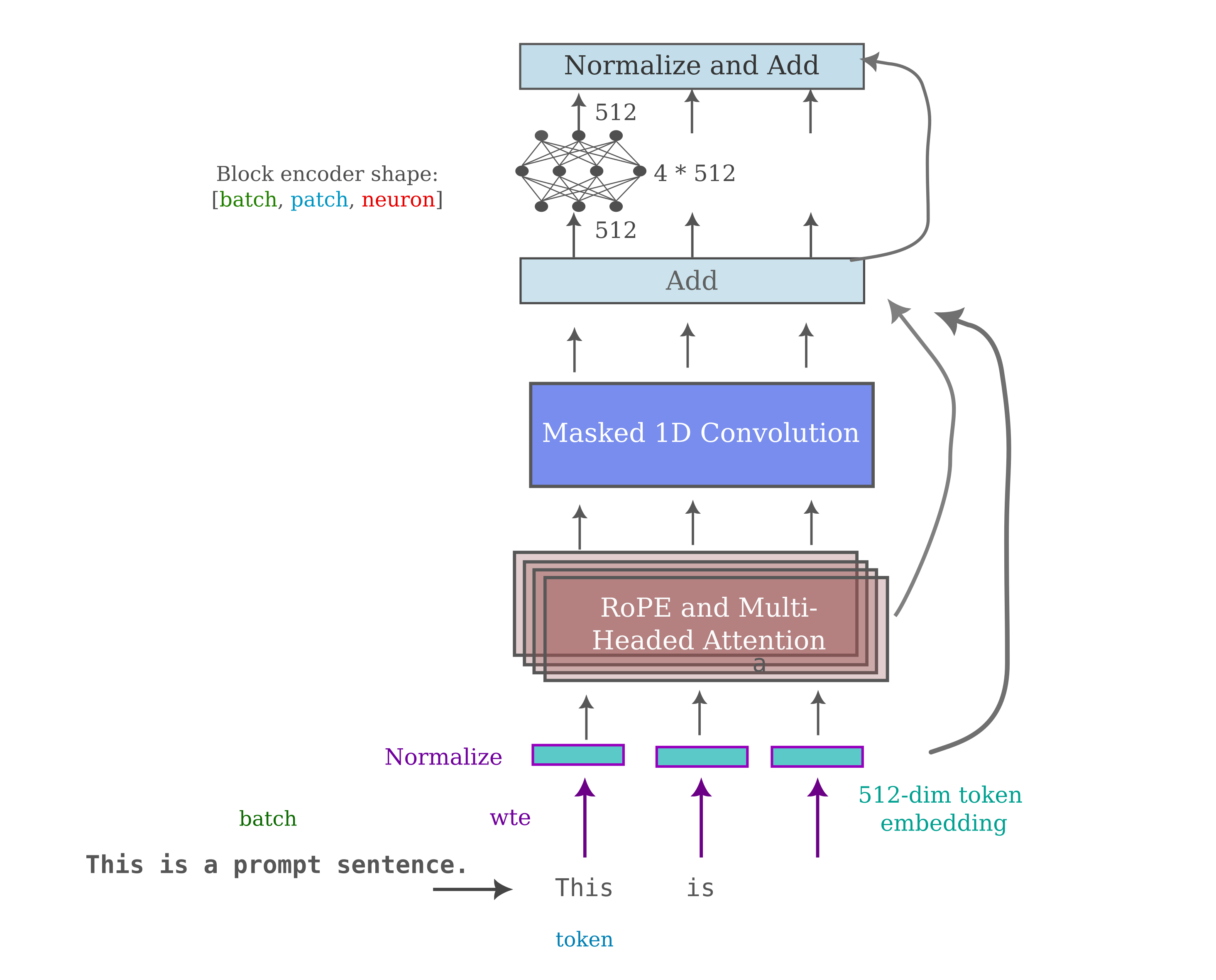
First, we define the operations on one mixer block, which is a module akin to one transformer block. The 1-dimensional convolutions that replace self-attention may be visualized as follows:
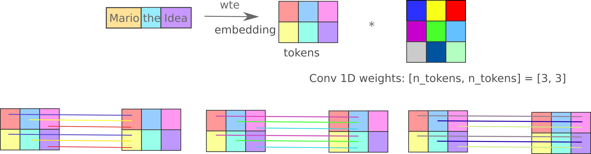
The kwarg expand_conv allows us to use this expansion or forego it for a single convolution (that must have as many output features as sequence elements). This is initialized as follows:
class MixerBlock(nn.Module):

	def __init__(self, dim, length, mixer_mask=True, expand_conv=True):
		super().__init__()
		self.patch_layernorm = nn.LayerNorm(dim)
		self.seq_layernorm = nn.LayerNorm(dim)
		self.dim = dim
		self.length = length
		self.patch_ff = FeedForward(dim)
		self.expand_conv = expand_conv
		if self.expand_conv:
			self.conv = ConvForward(length)
		else:
			self.conv = nn.Conv1d(length, length, 1)

		# for CLM training, apply lower triangular mask to convolution weights during the forward pass
		self.mixer_mask = mixer_mask
The last line of the code block above passes the boolean mixer_mask to a class variable to be accessed during the forward pass of the MixerBlock. What exactly this mask will look like will depend on whether we expand the inter-token convolution transformations or not, by which is meant mirroring the two-layer linear transformation (with nonlinear activation) that define the FeedForward modules. The similarities may be shown as follows:
def FeedForward(dim, expansion_factor=4):
	inner_dim = int(dim * expansion_factor)
	return nn.Sequential(
		nn.Linear(dim, inner_dim),
		nn.GELU(),
		nn.Linear(inner_dim, dim)
	)

def ConvForward(dim, expansion_factor=2):
	inner_dim = int(dim * expansion_factor)
	return nn.Sequential(
		nn.Conv1d(dim, inner_dim, 1),
		nn.GELU(),
		nn.Conv1d(inner_dim, dim, 1)
		)
where the ConvForward module is the transformation between tokens.
We will train the architecture using the masking approach that is commonly applied to causal language models in which the objective of training is to predict the next token in a sequence. This means that we need to prevent the model from using information from tokens to the right some token when learning to predict that token.
class LanguageMixer(nn.Module):

	def __init__(self, n_vocab, dim, depth, tie_weights=False):
		super().__init__()
		self.wte = nn.Embedding(n_vocab, dim)
		self.mixerblocks = nn.ModuleList(
			[MixerBlock(
				dim = dim,
				length = tokenized_length,
				)
			for i in range(depth)]
			).to(device)
		self.lm_head = nn.Linear(dim, n_vocab, bias=False)
		if tie_weights:
			self.lm_head.weight = self.wte.weight
		self.cel = nn.CrossEntropyLoss()
For a recursive neural network model, there is pretty much one way to train the model: for each word in a sequence, get the model’s prediction, find the loss, and backpropegate. For transformers and other models we could do the same thing but there is a much more efficient way to train: instead of iterating through all words in an input we instead feed the entire input into the model as if we were going to predict the next word, but instead we take the lm_head output for each input, find the loss, and backpropegate the total loss.
There are two important modifications necessary for this more parallelizable training. The first is that we need to have the model compare the output of the model for sequence elements $a_0, a_1, …, a_{n-1}$ to the element $a_n$ during the loss calculation, meaning that we need to shift the target element $a_n$ such that it is accessed when the model is at position $a_{n-1}$. This is accomplished in the forward pass of the model (below) by shifting the labels (the target elements) to start with the input element at index 1 rather than index 0 in labels[..., 1:].contiguous(). The model’s outputs are clipped such that the last output (which would correspond to the next element after the end of the input and does not exist in the input itself) is omitted. For compatibility with the HuggingFace trainer, we compute the cross-entropy loss in the forward pass and supply the value as part of a tuple with the output itself.
The line labels = rearrange(labels, 'b p t -> b (p t)') in the forward pass may be unfamiliar with those who have not worked with vision models in the past. For whatever reason, Einstein sum tensor manipulation never became as popular in the language modeling world as for vision models. There are certainly pros (succinct notation) and cons (portability) to using einsum notation, but we will use einsum mostly for reshaping tensors. For example, labels = rearrange(labels, 'b p t -> b (p t)') simply removes an index dimension of our tensor between the batch and token dimensions and could also be accomplished with labels = torch.squeeze(labels, dim=1) but is arguably more expressive.
class LanguageMixer(nn.Module):
	...
	def forward(self, input_ids, labels=None):
		x = input_ids
		x = x.to(device)
		x = self.wte(x)
		for block in self.mixerblocks:
			x = block(x)
		output = self.lm_head(x)
		labels = rearrange(labels, 'b p t -> b (p t)')
		output = rearrange(output, 'b t e -> b e t')
		shift_logits = output[..., :-1].contiguous()
		shift_labels = labels[..., 1:].contiguous()
		loss = self.cel(shift_logits, shift_labels)
		return loss, output
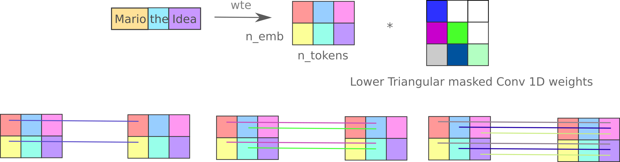
Besides shifting the output, we need a second addendum for causal language modeling: only information from previous tokens $a_0, a_1, …, a_{n-1}$ must reach token $a_n$ and not information from succeeding tokens $a_{n+1}, a_{n+2}, …$. For the transformer architecture it is customary to mask the softmax values of the $KQ^T$ to only use information from query projections of past tokens, but as we are using a 1-dimensional convolution transformation with no softmax a different approach will be necessary.
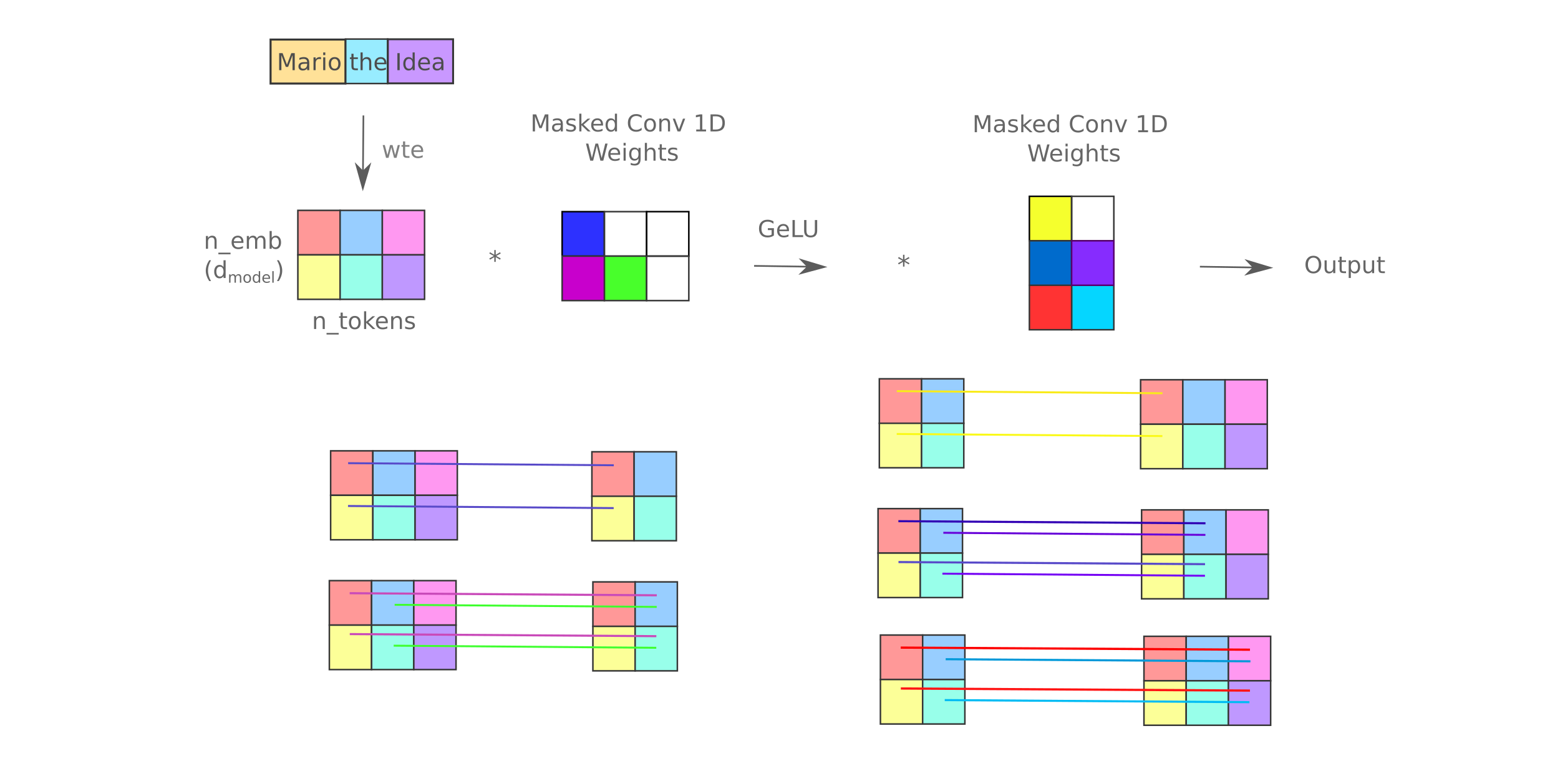
Instead we shall mask the weights of the convolution such that the only non-zero weights supplied to $a_n$ will originate from $a_0, a_1, …, a_{n-1}$. How this may be done is easier to see if we look at only one convolution between token: given an input matrix $X \in \Bbb R^{m, n}$ with $m=3$ tokens and $n=2$ features per token,
\[X = \begin{bmatrix} x_{0, 0} & x_{0, 1}\\ x_{1, 0} & x_{1, 1}\\ x_{2, 0} & x_{2, 1}\\ \end{bmatrix}\]if we are given convolution weights from a single filter layer
\[W_0 = \begin{bmatrix} 2\\ 1\\ 0\\ \end{bmatrix}\]we get the output (ie one token)
\[X * W_0 = \\ \\ \begin{bmatrix} 2x_{0, 0}+1x_{1, 0}+0x_{2, 0} & 2x_{0, 1}+1x_{1, 1}+0x_{2, 1}\\ \end{bmatrix}\]Likewise, with two convolutional feature weight layers we perform the same operation with the second to recieve a 2x2 output and for three we have a 3x2 output. If we concatenate the weight layers together in a single matrix such that each column weight becomes a matrix column, we want to use an upper triangular mask: in this case, the convolutional weight matrix $W$
\[W = \begin{bmatrix} 2 & 1 & 1\\ 1 & 1 & 4\\ 1 & 3 & 1\\ \end{bmatrix}\]becomes the masked weight matrix $m(W)$ upon Hadamard multiplication to an upper-triangular mask matrix $U$,
\[m(W) = W \circ U \\ m(W) = \begin{bmatrix} 2 & 1 & 1\\ 1 & 1 & 4\\ 1 & 3 & 1\\ \end{bmatrix} \circ \begin{bmatrix} 1 & 1 & 1\\ 0 & 1 & 1\\ 0 & 0 & 1\\ \end{bmatrix} = \begin{bmatrix} 2 & 1 & 1\\ 0 & 1 & 4\\ 0 & 0 & 1\\ \end{bmatrix}\]such that now for the first token we have the output
\[X * m(W) = \\ \begin{bmatrix} x_{0, 0} & x_{0, 1}\\ x_{1, 0} & x_{1, 1}\\ x_{2, 0} & x_{2, 1}\\ \end{bmatrix} * \begin{bmatrix} 2 & 1 & 1\\ 0 & 1 & 4\\ 0 & 0 & 1\\ \end{bmatrix} \\ \\ = \\ \\ \begin{bmatrix} 2x_{0, 0}+0x_{1, 0}+0x_{2, 0} & 2x_{0, 1}+0x_{1, 1}+0x_{2, 1}\\ 1x_{0, 0}+1x_{1, 0}+0x_{2, 0} & 1x_{0, 1}+1x_{1, 1}+0x_{2, 1}\\ 1x_{0, 0}+4x_{1, 0}+1x_{2, 0} & 1x_{0, 1}+4x_{1, 1}+1x_{2, 1}\\ \end{bmatrix}\]which is what we want, as each token recieves non-zero weights from preceeding (after shifting) tokens only.
In our implementation we actually use a lower-triangular mask (tril) because we must first re-arrange each convolutional weight tensor into a single weight matrix before Hadamard multiplication to the mask, and by default our rearrangement places each convolution weight column as a row in our collected matrix, ie it is transposed.
rearranged_shape = rearrange(self.conv.weight, 'f d p -> f (d p)').shape
mask = torch.tril(torch.ones(rearranged_shape)).to(device)
applied_mask = rearrange(self.conv.weight, 'f d p -> f (d p)') * mask # Hadamard mult to mask
self.conv.weight.data = rearrange(applied_mask, 'f (d p) -> f d p', p=1)
Thus we modify each 1D convolution in the mixer such that the convolutional weight is lower-triangular and perform the same operation as before,
We make it optional to use the original mixer architecture (where two 1D convolutions are applied sequentially between each pair of sequence elements) via the kwarg expand_conv, and for that we actually need to perform the reshaping and masking for both convolutions. The architecture with only one convolution between sequence elements we call the ‘flat’ mixer, as it must have a fixed number of convolutions to sequence length elements. The mask is applied during the forward pass as follows:
class MixerBlock(nn.Module):

	def __init__(self, dim, length, mixer_mask=True, expand_conv=True):
		super().__init__()
		...

	def forward(self, x: torch.tensor):
		if x.dim() > 3:
			x = rearrange(x, 'b p t f -> (b p) t f')

		# for CLM training, apply lower triangular mask to convolution weights
		if self.mixer_mask:
			# Mask logic here
			...
		residual = x
		x = self.seq_layernorm(x)
		x = self.conv(x) + residual
		residual = x
		x = self.patch_layernorm(x)
		x = self.patch_ff(x) + residual
		return x
Note that it is tempting to skip a step and simply apply the triangular mask directly to the convolution weights by re-assigning the parameters of those weights to masked values of the original weights. This leads to a tricky problem after backpropegation: the original weights will not be updated! The optimizer (here AdamW) takes as an argument the model as it is initialized, but the parameters after masking during the forward pass are newly initialized at this time and will not be recognized by the optimizer.
Finally, we use a dataset amenable to small models: the TinyStories dataset, which we truncate to 2M ‘stories’. A Llama-style tokenizer with 4096 unique tokens was trained on this dataset and used for both transformer and mixer models during training and inference.
Training
We make use of the transformers.trainer() module, which has a couple very useful features for ease of use: automatic logging checkpointing the model and optimizer states, masking loss on the pad token, 16 bit mixed precision numerical stabilization to name a few. For testing purposes one can also used the following barebones trainer (note that this does not mask pad token loss and should not be used for an actual training run):
def train_model():
	model.train()
	total_loss = 0
	for step, batch in enumerate(train_data):
		batch = rearrange(batch, 'b (p t) -> b p t', p=1)
		optimizer.zero_grad()
		batch = batch.to(device) # discard class labels
		loss, output = model(batch, batch)
		total_loss += loss.item()
		loss.backward()
		optimizer.step()
	print ('Average loss: ', total_loss / len(batch))
To make results comparable, we use the same tokenizer, dataset (TinyStories), and batch size (16) and observe the training and evaluation cross entropy loss for the transformer model (Llama, whose source code may be found here) compared to our model. This new model is dubbed the ‘masked mixer’, both because the model masks convolutional weights during both training and inference and because some versions of this model are not fully-MLP architectures at all but utilize convolutions of size greater than 1 between tokens. We perform training runs of around 12 hours on an RTX 3060 unless otherwise noted.
It should first be stated that the transformer requires substantially more memory to store the gradients, optimizer, and parameters than the mixer: given a batch size of 16, a llama model with $d_{model}=128$ and $n=8$ exceeds 10 GB vRAM during training compared to the 2.4 GB vRAM required for a mixer of the same $n$ and double the $d_{model}$, both for a context window size of 512. This is due to inefficient memory usage for that model size (transformers with a width of less than 256 are poorly allocated in memory), but for larger $d_{model}$ values the large amount of memory required stems from the increased number of non-trainable inter-token parameters necessary for backpropegation in the transformer compared to the mixer.
It is also apparent that transformers are much slower to train than mixers. This results from both the number of effective parameters (above) and also from the more efficient use of gradient flow by the mixer, as gradient do not need to pass along non-trainable parameters as is the case for transformers (where attention gradients travel from $K,Q,V$ projections to the $K,Q,V$ values themselves and back as well as softmax transformations etc). Thus we cannot compare these models directly using only $d_{model}$ and $n$, but instead use a ballpark figure for these and compare training and test vRAM.
Because of this, optimizing a mixer of a similar size to a transformer requires much less compute: one typically sees between 10x and 20x the time required for a transformer with $d_{model}=128$ and $n=8$ compared to a mixer with twice the $d_{model}$ and the same number of blocks for the same forward and backpropegations steps.
Now we train the models using an approximately fixed compute budget (12 GB vRAM and 12 hours on an RTX 3060). We find that the masked mixer with the parameters detailed above achieves a substantially smaller training (2.169) and validation (2.201) loss (Cross-Entropy loss, equal to $\log_2 \mathrm{perplexity}$) after this twelve hours than the Llama model (2.497 validation and 2.471 training loss). This is mostly because the mixer is around six times as fast to train as the transformer: there is nearly identical loss if we compare equal steps (2.497 versus 2.505 validation loss at step 160000). Equivalent steps mean little for language models, however, as they are inherently resistant to overfitting (see that there is minimal overfitting after 5.6 epochs at twelve hours of training for the mixer) such that simply increasing the dataset size or number of epochs in this case yeilds lower training and validation loss than training a larger model with an effectively smaller dataset.
Mixer Inference
Low training and validation loss are useful guides of efficacy, but the goal of this research is to find architectures that are more efficient than the transformer at causal language modeling, which is simply to generate the next word in a sentence.
It is tempting to simply take the last output of the mixer model as the next token and perform a sliding window on the input to keep a constant number of tokens (which the mixer requires, unlike a transformer model). But there is a problem with this method: the last output is not actually trained at all! Recall that the model used a shifted logits approach, such that the trained output is $[…, :-1]$ which does not include the last element because that is the prediction for the next token after the input ends, information that is absent.
Instead we can have the mixer simply replace token after token, maintaining the causal language mask after the last supplied token as follows:
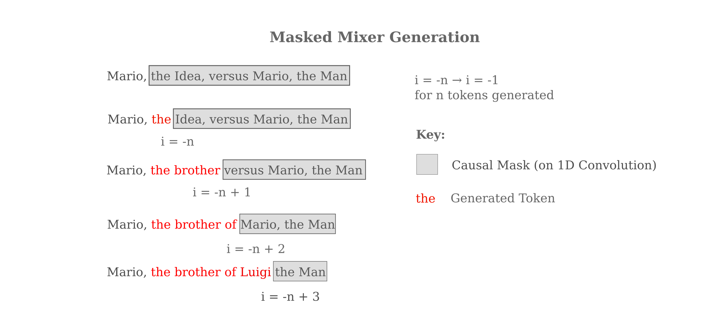
For 50 generated tokens at the end of the 512-length context window, this corresponds to the following inference code:
fout = []
for i in range(50, 1, -1):
	loss, output = model(tokens, labels=tokens)
	out_token = torch.topk(output, dim=1, k=1).indices.flatten()[-i]
	tokens[..., -i+1] = out_token
while maintaining the mixer_mask=True flag on the model.
The outputs are extremely good: for our mixer of size $d_{model}=256$ and $n=8$ blocks (1.8 GB vRAM for 16-bit training on 512 context tokens), trained for 12 hours on TinyStories, we have for the validation dataset input (<unk> tokens are newlines)
”””
Once upon a time, there was a little boy named Tim. Tim had a big, orange ball. He loved his ball very much. One day, Tim met a girl named Sue. Sue had a pretty doll. Tim liked Sue’s doll, and Sue liked Tim’s orange ball.
The actual next 50 tokens to this input (generated by ChatGPT) are
”””
want.” Tim said, “I promise to take care of your doll too.”
and our language mixer supplies the following output:
come back."<unk>Tim thought about it and agreed. Sue gave the ball back to Tim. They played together, and Tim was very happy. Sue was happy too. They learned that sharing can make everyone happy. And that is how the orange ball can bring happiness to everyone.
Compare this to the greedy generation output from the Llama transformer model $d_{model}=128$ and $n=8$ blocks (10.7 GB vRAM for 16-bit training on 512 context tokens), trained for 12 hours on TinyStories:
'll find your ball."<unk>Tim was happy. He said, "Thank you, Sue. You are a good friend. You are a good friend." Sue gave Tim a new ball. Tim gave Sue a new ball. Sush was blue and shiny. Sush, Spot, and Spot. They played with their ball
although this turns out to be a bad prompt for the transformer. A better one is as follows:
”””
One day, a little boy named Tim went to play with his friend, Sam. They wanted to play a game with a ball. The game was to see who could get the best score.
The masked mixer completes this story as follows:
played a game of tag. Tim was fast, but Sam was faster. They ran and ran until they reached the finish line. Tim was tired but happy. Sam said, "Good job, Sam!" Sam smiled and said, "Good job, Tim!" They both smiled and hugged each other.
The transformer completes this as
went home. They sat down on the grass and closed their eyes. They closed their eyes and fell asleep. Tim dreamed of the snow he found his way home. He felt safe and happy in his new score. He knew that he could always count on his score again. And he lived happily ever after.
which is a little less coherent. Thus we see that there is indeed an improvement in output quality, reflective of the lower training and evaluation loss of the trained mixer compared to the transformer.
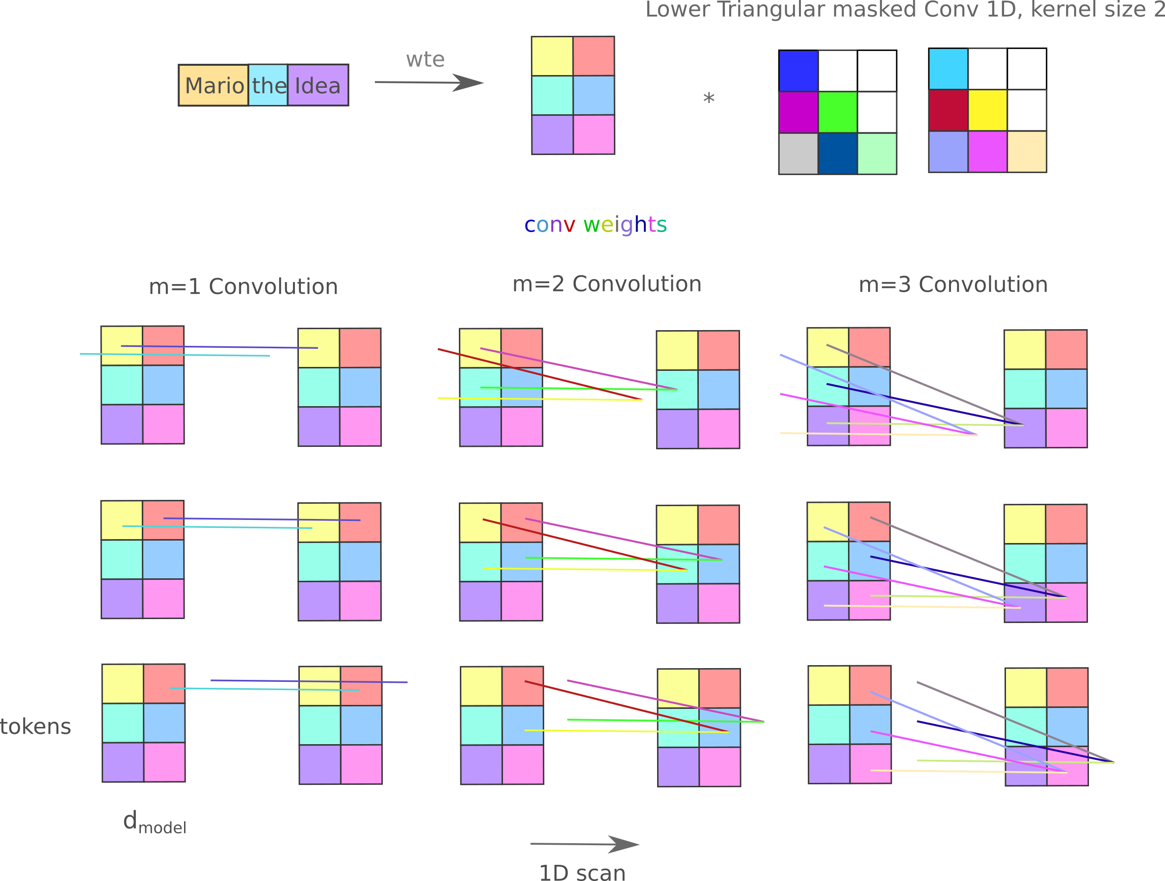
Flat Mixers Train Faster
When examining the ability of various model to represent their inputs, it was found that representation of tokens whose output was masked (indicative of the amount of information transfer between tokens) is accurate for untrained masked mixers if either the model were relatively large ($d_{model}=1024, \; n=24$ or $d_{model}=2048, \; n=8$) or else if the model remained small $d_{model}=512, \; n=8$ but the expanded sequential convolutions were replaced with a single convolution as shown in a previous section on this page.
This suggests that these ‘flat’ mixers may be able to be trained more effectively than the expanded convolution mixers or transformers, and experimentally this is indeed the case: a $d_{model}=512, \; n=8$ flat mixer (requiring 3.59 GB vRAM to train on a context window of 512 tokens) achieves a training loss of 1.842 and a validation loss of 1.895 after 12 hours on TinyStories, which is lower than the $d_{model}=256, \; n=8$ transformer that requires more than double the memory (1.99 and 2.03 training and validation, respectively).
Flat mixers experience superior training characteristics compared to two-layer ‘expanded’ mixers as well: depending on the expansion factor, the latter’s sample throughput is 20-50% smaller. Which expansion factor should one use? If we consider how the causal language weight mask for this particular implementation, it is clear that there is only one expansion that makes sense: the 1x expansion in which the hidden layer is the same dimension (ie the sequence length) as the input and outputs. This is because the lower-triangular mask negates all ‘extra’ weights for any expansion greater than a factor of one, as is apparent in the following figure.
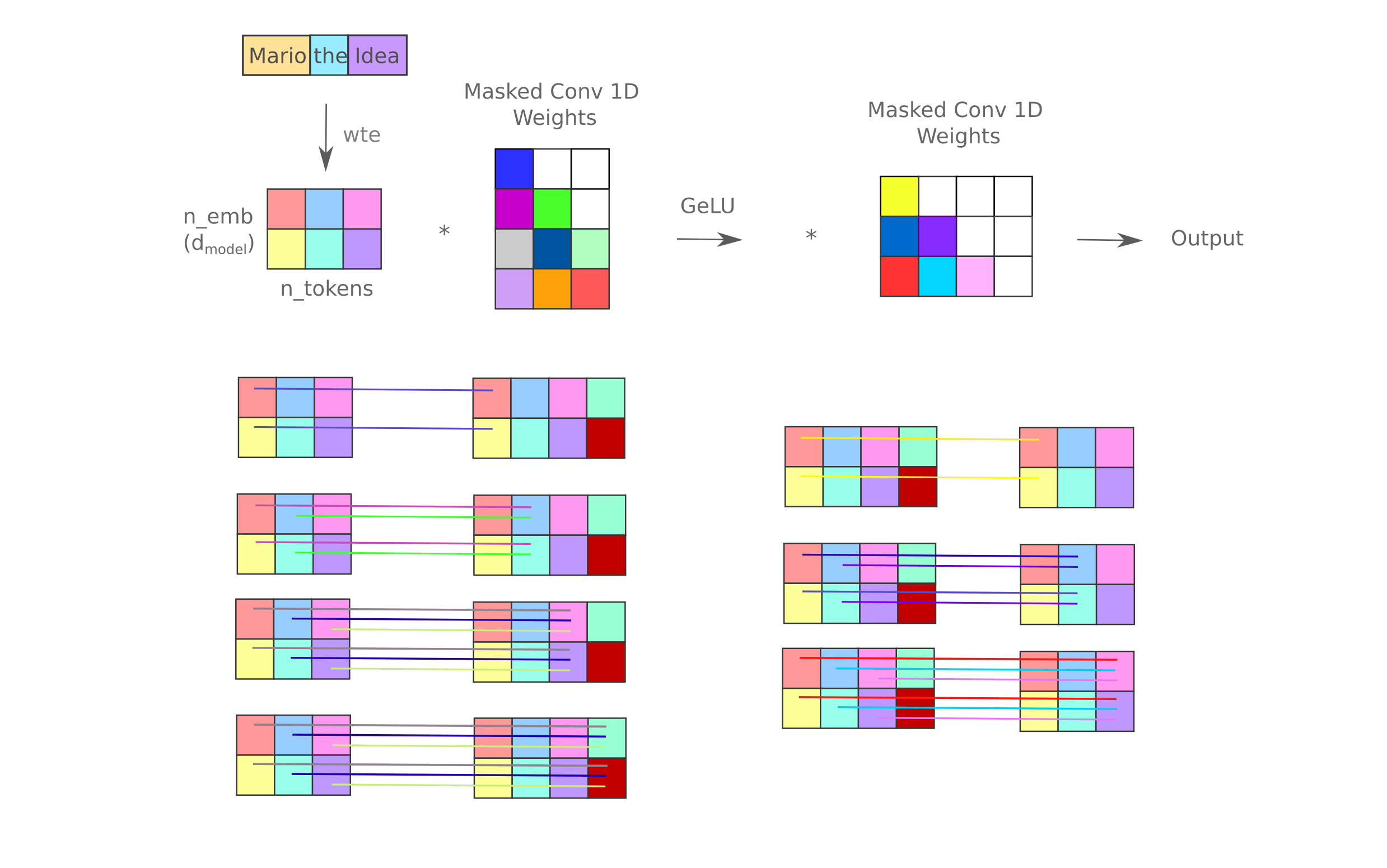
The situation for any mixer with an expansion factor of less than one is even worse: here input components after a certain index are lost due to the causal language mask. It might be wondered if one could simply not mask the first convolution and mask the second to avoid this issue, but that would cause information from later tokens to influence earlier tokens (even with the second convolution being masked) and thus is not a viable approach.
Even disregarding the time and superfluous parameters, however, expanded mixers of the same $d_{model}, n$, context, and batch size achieve larger loss even for a fixed number of samples seen. For example, a $d_{model}=512, \; n=8$ mixer with an expansion factor of 2 achieves a training and validation loss of 2.159 and 2.183 compared to the flat mixer’s 2.087 and 2.111 after one epoch. This is counterintuitive given that the expanded mixer has more inter-token trainable parameters than the flat mixer such that one might expect this architecture to achieve lower per-sample loss (even if it trains more slowly), and in the author’s opinion is best appreciated from the point of view of the superior nonself-token representation of flat mixers.
It may be wondered if the performance increase in masked mixers compared to transformers is only due to the relatively small size of the transformer models tested thus far, and if larger transformers would be better learners than larger mixers. The largest 8-layer transformer that will fit in 12GB vRAM (at 512 token context with a 16-size minibatch) has a $d_{model}=256$, and at 12 hours on a 3060 this achieves 1.99 and 2.03 training and validation loss, respectively. This lags behind the training and validation loss of 1.81 and 1.86 of a $d_{model}=1024, \; n=8$ mixer trained with the same total compute budget.
If one is able to vary the batch size, larger transformers and mixers still may be tested. A transformer of size ($d_{model}=512, \; n = 8$) with a batch size of 8 can just barely fit in the allotted 12 GB vRAM and this model achieves a peak of efficiency for the transformer architecture on this test, reaching training and validation losses of 1.873 and 1.908, respectively. We can consider this to be something near to a peak transformer model performance because if the model is further enlarged to $d_{model}=1024$ (which requires a reduction to a batch size of 4 for our vRAM stipulations) then performance suffers dramatically, reaching only 2.313 and 2.315 training and validation loss at the end of one training run. The larger transformer underperforms even when one focuses on the loss after a particular number of images seen: after 440k images, the $d_{model}=1024$ transformer has a training loss of 2.315 but the $d_{model}=512$ transformer reaches a training loss of $2.078$.
Even for the optimal $d_{model}$ for the transformer at ($512$) the flat masked mixer achieves lower losses (1.842 and 1.895). When we compare a masked mixer with a smaller effective size ($d_{model}=1024, \; n = 8$) and are free to increase the minibatch size to 32 samples (the largest power of two that fits in the allotted 12GB vRAM), we achieve substantially lower losses once again: 1.784 and 1.837 train and validation, respectively.
To sum up, flat mixers achieve lower training and validation loss than either llama-style transformers or expanded mixers, which follows from the superior self- and nonself- token representation present in these models.
Testing on inference bears out the cross-entropy loss findings: given the same prompt in the last section (“One day, a little boy…”), the trained $d_{model}=1024, \; n=8$ flat mixer yields
played a game of catch. Tim threw the ball to Sam, and Sam caught it. They laughed and played until the sun went down.<unk>At the end of the day, Tim and Sam were tired but happy. They went home and took a nap. They dreamed of playing catch again tomorrow. And they did.
which is a more coherent and plot-accurate completion than either the transformer or even the expanded mixer presented in the last section of this page, again reflective of a lower training and validation loss than either architecture.
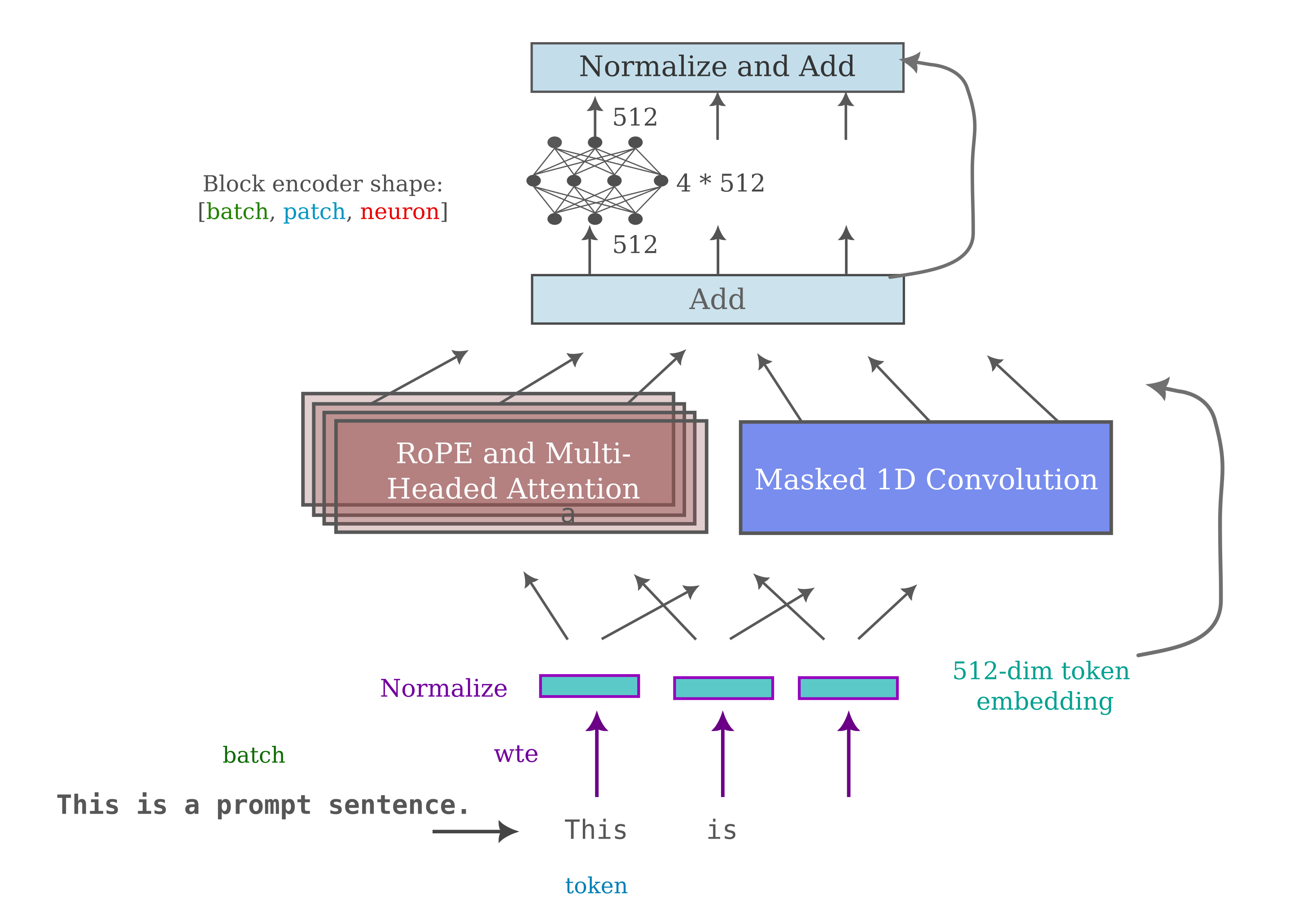
Parallel rather than Sequential Convolutions
We have seen that the original mixer architecture with two 1-Dimensional convolutions sequentially (and GELU inbetween) learns language much more slowly than a mixer with only one 1-Dimensional convolution between sequence elements.
This observation presents a certain difficulty in that the 1D convolution must have as many filters as sequence elements squared to map a sequence to itself (all to all), meaning that the inter-sequence weights scale with sequence length but not the $d_{model}$. This is not necessarily a problem for performance, as it is clear that simply increasing the $d_{model}$ yields increased asymptotic performance.
What if we do want to increase the number of inter-sequence weights? According to studies on representation accuracy, replacing multiple convolutions in series with sets of convolutions in parallel is the solution: both self- and non-self token representation is superior to either expanded or mixers. In the following diagram, we replace one convolution with two parallel ones,.
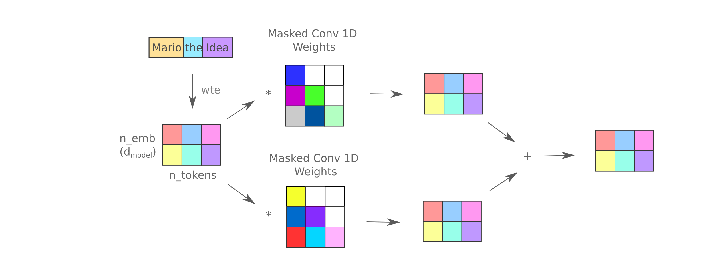
For a given number of training updates, the 2-parallel convolution mixer results in lower loss for a $d_{model}=512, n=8$ mixer: 1.845 versus 1.886 training loss at 354,000 steps (the most this model can finish in our fixed compute training). However, as the model is slower to train per step it does tends to reach a very similar or perhaps slightly worse fixed-compute loss as the flat mixer of the same $d_{model}$ (1.842). Increasing the number of parallel convolutions to 4 leads to no apparent fixed-compute loss reduction either.
Mixers do not benefit from positional encoding
By learning values for each combination of two tokens, the masked mixer learns an implicit absolute positional encoding and would not be expected to benefit from more positional encoding information. We can provide positional information in the form of a simple one-element addition to the first block’s input vector as follows:
class LanguageMixer(nn.Module):

	def __init__(self, n_vocab, dim, depth, tokenized_length, batch_size, tie_weights=False):
		...
		self.positions = torch.arange(-tokenized_length//2, tokenized_length//2, 1).to(device)

	def forward(self, input_ids, labels=None):
		...
		tokenized_length, batch_size = x.shape[-1], x.shape[0]
		positional_tensor = rearrange(self.positions, '(s b) -> s b', b = tokenized_length).unsqueeze(0).unsqueeze(-1)
		positional_tensor = positional_tensor.repeat(batch_size, 1, 1, 1)
		x = self.wte(x)
		x = torch.cat((x, positional_tensor), dim=-1)
		positional_tensor = positional_tensor.squeeze(1).squeeze(-1)
		x[..., -1] = positional_tensor
		for block in self.mixerblocks:
			x = block(x)
		output = self.lm_head(x[..., :-1])
but after doing so we see virtually no change in performance after our one unit of compute has been applied. If we instead apply the positional information to every block via
		for block in self.mixerblocks:
			x = block(x)
			x[..., -1] = positional_tensor
we see detrimental effects on training: our final loss is 1.94 train and 2.10 eval.
Scaling Properties
The masked mixer architecture gives us an easy way to modify the number of inter-token weights (1D convolution ConvForward weights) as well as the number of intra-token weights (the FeedForward weights). We can observe the loss achieved by varying the number of each type of parameter independently, a feat which is much more difficult to pull off for the transformer as the number of $K, Q, V$ projection weights are usually tied to the $d_{model}$.
Which type of weight is likely to be more important: that is, given a fixed number of total weights should we allocate more to intra- or inter-token parameters for the lowest loss given a fixed amount of compute? When considering the causal language generation process, there are arguments to be made for both types, as clearly complex relationships between words are just as important if not moreso than a nuanced understanding of a word itself.
One argument for the importance of allocating more parameters to intra-token weights is that all information from all previous words must pass through these weights (ignoring residual connections for the moment), whereas inter-token weights may add information from many parts of an input over many layers.
”””
One day, a little boy named Tim went to play with his friend, Sam. They wanted to play a game with a ball. The game was to see who could get the best score.
This can be seen when we compare the completion of a 64-dimension model with 64 layers, which achieves a 2.867 evaluation loss after a training run,
played. They saw a man who had fallen down the street. Tim said, "Time to go home, please." Tim said, "It's okay to be scared, but we have to be careful." Tim nodded and they went home. They played in the big field and had fun. They had a great time playing in the snow.
which is gramatically correct but loses the train of the story (Sam is forgotten, playing outside after going home, snow appearing etc.) which is typical of models of that dimension. On the other hand, a 1024-dimension model with 8 layers reaching a evaluation loss of 1.837, which gives the much more coherent
played a game. They took turns throwing the ball to each other. Tim was good at catching the ball. Sam was good at catching the ball. They laughed and played until it was time to go home.<unk>The moral of the story is that playing games is fun, but sometimes it's good to try new things and have fun with friends.
The following table provides a summary of the results of transformer, expanded mixer, and flat mixer performance after one unit of compute (12 hours on an RTX 3060) applied to the first 2M examples of TinyStories:
Transformer ($n=8$ layers, $h=16$ attention heads, $b=32$ batch size unless otherwise noted):
| $d_{model} = 128$ | $d_{m}=256$ | $d_{m}=512$ | $d_{m}=1024$, b=8 | |
|---|---|---|---|---|
| Train | 2.38 | 1.99 | 1.87 | 2.31 |
| Test | 2.40 | 2.02 | 1.91 | 2.32 |
with the flat mixer (n=8, b=16)
| $d_{model} = 256$ | $d_{m}=512$ | $d_{m}=1024$ | $d_m=1024$, b=32, n=4 | $d_{m}=2048$ | |
|---|---|---|---|---|---|
| Train | 2.11 | 1.84 | 1.81 | 1.78 | 2.05 |
| Test | 2.15 | 1.89 | 1.86 | 1.84 | 2.07 |
And for the expanded mixer (n=8, b=16),
| $d_{model}=256$ | $d_{m}=512$ | $d_{m}=1024$ | |
|---|---|---|---|
| Train | 2.17 | 2.05 | 1.83 |
| Test | 2.20 | 2.08 | 1.89 |
We can also consider the memory scaling with respect to the number of tokens in the context length, $n_{context}$. It is apparent that both the transformer and masked mixer have the same computational complexity as length increases because every token is operated on by every other token for both models (resulting in an $O(n^2)$ space complexity). But it is also apparent that the flat masked mixer has a much lower constant factor for this scaling than the transformer, as each token-token operation consists of far fewer mathematical operations. When the memory required (in megabytes of vRAM, beyond 12 is OOM) to make an unbatched forward and backward pass (without a language modeling head) for a $d_m = 1024$ flat masked mixer,
| $n_{context} = 512$ | $n_{c}=1024$ | $n_{c}=2048$ | $n_{c}=4096$ | $n_{c}=8192$ | |
|---|---|---|---|---|---|
| $n_{layers}$ = 4 | 2071 | 2341 | 2637 | 3573 | 6491 |
| $n_l=8$ | 2431 | 2869 | 3425 | 5111 | 10527 |
| $n_l=16$ | 2695 | 3159 | 3811 | 5879 | OOM |
is compared to that for a transformer of the same width, we see that the masked mixer is around four times as memory-efficient with increasing token length.
| $n_{context} = 512$ | $n_c=1024$ | $n_c=2048$ | $n_c=4096$ | $n_c=8192$ | |
|---|---|---|---|---|---|
| $n_{layers} = 4$ | 2323 | 3275 | 6809 | OOM | OOM |
| $n_l=8$ | 3176 | 4800 | 10126 | OOM | OOM |
| $n_l=16$ | 4876 | 7750 | OOM | OOM | OOM |
One might wonder why the masked mixers is so much more memory-efficient to train given that training requires modification of parameters, and transformers have only very slightly more parameters than mixers of the same $d_m$. The answer is that when training deep learning model architectures typically applied to language and vision modeling tasks (such as transformers and convolutional models) most device memory is taken up by activations, rather than parameters. Unless gradient checkpointing is applied (which re-computes activations rather than saving to global device memory at the cost of significantly lower throughput), we must save every activation a model generates during the forward pass in order to be able to backpropegate the training loss across. To be specific, between any weight layers there is usually an activation function, an activation layer, and possibly a normalization operation. When the gradients are formed on the second of the two weight layers, we must first backpropegate to the activation layer before backpropegating to the first weight layer but if we don’t know the activations then we cannot form the gradients on the activation layer.
This is important because masked mixers have far fewer activations related to inter-token operations than transformers: for the flat masked mixer, we essentially have no purely inter-token activations (as we convolve over $d_m$ activations at each layer which must already exist) whereas the number of activations for a transformer is $(n(k * h) + n(q * h) + n(v * n)^2$ where $n(k)$ denotes the size of the activations in a given projection, $h$ the number of self-attention heads, and $q, k, v$ the key, query, and value projections.
From this analysis it is clear that although mixers and transformers both are $O(n^2)$ space complexity for $n$ tokens, masked mixers are far more efficient in practice due to their smaller constant factors denoting the number of activations necessary for each next token. The same is true of the FLOPs required for each model type during training, as the ratio of memory access to compute for backpropegation across the activations is a low constant factor (perhaps 4:1). For this reason, masked mixers of twice the $d_m$ of a transformer are usually approximately equivalent with respect to both memory and computational throughput.
Transformers with fewer attention heads are more efficient for TinyStories
The observation that the flat mixer performs better than transformers on TinyStories completion given limited compute suggests that perhaps we can get similar performance from transformers if the inter-token information transfer is simplified. We have been using 16-headed attention, which corresponds to 16 parallel linear transformations making key, query, and values for each token. We can simply reduce this number by supplying the desired $n$ number of attention heads as follows:
llama_config_kwargs = {
    ...
    'num_attention_heads': n,
}
Conceptually this may be thought of as changing the number of simultaneous combinations of previous tokens’ value vectors that the model ‘considers’ for each next token. A single-headed attention model would be somewhat similar to a flat mixer, as each would have a single value corresponding to the attention between any two tokens. The best-performing 16-head attention transformer was $d_m=512, n_l=8$ and when we reduce the number of attention heads while keeping the compute the same, we have the following for 12 hours of 3060:
| $n_{heads} = 16$ | $n_h=8$ | $n_h=4$ | $n_h=2$ | |
|---|---|---|---|---|
| train loss | 1.87 | 1.70 | 1.66 | 1.68 |
| eval loss | 1.91 | 1.77 | 1.71 | 1.73 |
The main reason for this performance increase is that the smaller number of attention heads results in more samples seen during training in a given compute budget: for example, if we compare the loss after a fixed number of inputs seen we find that the 2-headed attention is not as effective as the 16-headed attention, at 1.96 train and 1.98 eval for two heads versus 1.87 train and 1.90 eval loss for 16 heads after half an epoch.
It might be wondered if this more efficient transformer might have better input representation, but we find that the opposite is true: neither at the beginning of training (where 16-headed attemtion transformers have fairly accurate one-block representation) nor at any other step during training does the two- or four-headed attention model exhibit anything remotely resembling accurate representation.
Fully Convoluted Mixers for optimal TinyStories training
The results in the last section seem to indicate that representational power is more important than representational accuracy, as a transformer model that has poor input representation accuracy and many inter-token parameters outperforms mixer models with extremely accurate input representation but fewer inter-token parameters. This is not necessarily the case, however, as a mixer-derived model with an increased number of inter-token parameters is capable of performing on par even the highly optimized transformer as we shall see in this section.
The hypothesis here is that the mixer model can ‘soak up’ larger learning rates than the transformer because it is in most cases easier to optimize once training has proceeded a good ways: the difficulty of accurate back-propegation for transformers is documented elsewhere, but mixers typically do not seem to suffer from these problems. Thus we increase the learning rate of the mixer and repeat the experiments for this model (with 8 layers and a $d_m=1024$ and a batch size of 32).
We can observe scaling properties of these models by training them with a much larger and more powerful compute cluster: a 4x V100 server. We train via Distributed Data Parallel, an algorithm that places replicas of the entire model of interest on each GPU and distributes data to each device, before all-gathering the gradients for backpropegation. This means that the effective batch size increases by a factor of 4 compared to the single-GPU training undertaken above, such that instead of say 32 samples per batch we have 32 samples on each of 4 gpus for 128 samples per gradient update total. Large language models are typically trained using modifications of the distributed data parallel algorithm, as these models cannot typically be held entirely in a single GPU’s memory. To make results somewhat comparable with the 12 hours on a 3060, we limit training times to 2.25 hours on the 4x V100.
For clarity, the mixer architecture is detailed in the following figure:
In contrast to the paralleled convolutions explored earlier, the convolutional kernal acts on the $d_{model}$ index, not the token index. The number of inter-token trainable parameters is equal to the kernel size multiplied by the number of weights in the 1D convolution of kernel size 1 (the number of sequence elements squared divided by two for masked mixers).
With this training protocol, the 4-headed, 8-layered llama model achieves a training (causal language model) loss and validation loss of 1.78 and 1.82, respectively. With the larger learning rate of $\eta=0.005$ this is slightly reduced to 1.76 and 1.79 training and test accuracy. This is far worse than what is achieved for a 8-layer, 4-sized convolution masked mixer (with the increased learning rate) which achieves training and validation losses of 1.62 and 1.74 given the same amount of compute. If we further optimize the transformer by increasing the batch size to 32, the transformer achieves nearly the same accuracies (1.68 and 1.73 respectively). If the mixer is modified slightly to contain an extra linear layer after the word-token embedding, the cross-entropy losses are 1.61 train and 1.71 test.
The main finding here is that a compute- and dataset-optimized mixer is generally slightly more performant than a similarly optimized transformer (notably without Flash Attention 2).
Multi Headed Mixers
As more than one self-attention head increases the learning efficiency for transformers, it may be wondered if increasing the number of mixer ‘heads’ would also lead to a concomitant increase in mixer learning efficiency. One may implement masked mixer heads in a number of ways but we choose to use a formulation similar to the original transformer. Each head is projected by a unique weight matrix and then a unique mixer is applied to each head, and the outputs are concatenated and then re-projected back to match the $d_{model}$ dimension. The following diagram portrays this approach for the case where each head’s convolutional kernal is of size one.
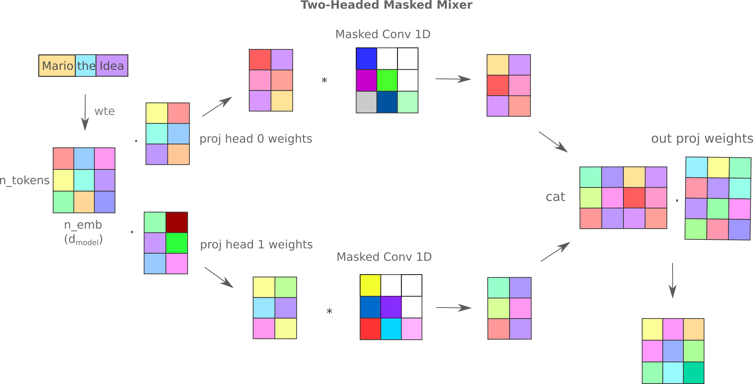
This approach yields a slight increase in training efficiency relative to the standard flat masked mixer with convolutional kernel of size 4: training/test losses for 2.25h on 4x V100 are 1.60/1.72 for the two-headed mixer versus 1.62/1.74.
Transformer mixer hybrids
The observation that mixers appear to learn a fundamentally different structure than transformers when applied to the same dataset suggests that they may act orthogonally (with some slight abuse to the linear algebraic phrase). This means that the abstract quantities a mixer learns might be complementary to those that a transformer learns, such that combining these architectures in some way might lead to a model that is a more efficient learner than either mixer or transformer alone.
Can adding a mixer component to a transformer or vice versa increase training efficiency? One way to implement this is as follows:
Recall that the 4-headed, $d_m=512$ transformer model achieved an train/test accuracy of 1.66/1.71 on TinyStories with 12 hours of RTX 3060 compute time, whereas the flat mixer with the same $d_m$ achieved values of 1.84 and 1.89, respectively. If these models learned the same way one would not expect for a composite model to outperform the transformer, but a quick test observes that it does: a transformer-mixer (with a flat mixer applied with a convolution size of one) hybrid achieves an accuracies of 1.62 and 1.67 given the same compute limit.
Scaling up the compute power via the 4x V100, we find that this transformer-mixer hybrid once again outperforms the transformer: for 2.25 hours on a 4x V100 node the hybrid achieves lower training and test loss than either mixer or transformer (above) with values of 1.53 and 1.59, respectively, which compares to train/test losses of 1.55 and 1.61 without the masked convolution (both with Flash Attention 2).
Another way to add mixer elements to a transformer is as follows: we instead add the mixer in parallel with the self-attention module. This does not yield any benefit from the standard transformer architecture, however, and achieves the same 1.55 and 1.61 loss values on the 4x V100 cluster (with flash attention 2). It turns out that swapping the order detailed above also does not improve CEL relative to the transformer.
It seems strange that the precise ordering of self-attention versus convolution should affect the model training abilities, and with further investigation the cause of this is revealed. It is even stranger that these effects are only observed using left padding during training and not right padding. A clue to this is what is observed in a sample-by-sample manner: we see that certain inputs that add a critical number of pad tokens preceeding the word tokens in the padding process result in a cross-entropy loss of 0! This is a sign of next token information being passed to the current token, and sure enough the Huggingface Llama implementation uses transformer modules that re-shape left-padded inputs for efficiency. This can clearly be beneficial if one does not calculate attention on pad tokens that follow an input (ie left-padding is swapped for right-padding) but results in the masked mixer triangular mask not matching the input properly. This accounts for the low CEL for transformer-mixer hybrids for left-padded inputs but not right-padded ones as well as the zero loss for certain (highly-padded) inputs as well as why swapping the order of attention and mixer layers leads to no benefit in training efficiency.
To conclude, there is actually no increase in model efficiency when masked convolutions are added before, in parallel to, or after attention in a Llama-style transformer.
Masked Mixers outperform early CLM Transformers
It should be noted that masked mixers are far more efficient learners than the original causal language modeling-style transformers, that is, before the introduction of optimizations like Rotary Positional Encoding and Flash Attention. This can be shown by comparing an early CLM style transformer’s learning on the TinyStories dataset to the mixer: for the OpenAI GPT implemented in the transformers library, the train/test accuracy achieved after 12 hours of 3060 compute is 2.04/1.96 using the optimized learning rate and $d_{model}$ values found for llama-style transformers. This is far worse than the 1.76/1.81 mixer loss, which is lower even than a GPT implementation with an optimized number of heads (1.96/1.89).
If a community were given seven years to optimize the performance of masked mixers and if the causal language modeling performance of this model were to generalize to larger datasets, it is in the author’s opinion very likely that masked mixers would out-perform even the most recent and highly optimized transformers. One could characterize the difference between masked mixer and transformer as being analagous to the x86-68 processor architecture compared with RISC-V: the latter is superior to the former given a constant amount of work in the field, but currently less effective as there have been so many optimizations on the x86 instruction set and architecture.
Accurate Representation and Retrieval
In some sense it is unsuprising that the transformer has relatively poor input representational accuracy compared to the masked mixer. After all, this architecture was design on the principle that some input words are more important than others for sequence-to-sequence tasks such as machine translation; these more important words receive more attention. The softmax-transformed dot product attention serves to effectively limit the number of input tokens that influence an output per head, and with multiple heads more of the input may be attended to for any given output. But for accurate input representation we want something entirely different: a sampling of all input elements with some mixing process such that the information in the hidden layers of the model for token $n$ may recapitulate the prior tokens $0, 1, …, n-1$. This is exactly what the mixer does.
But if transformers exhibit inaccurate input representation but are effective language task learners, does input representation accuracy really matter for causal language generation? These results seem to imply that transformational power (ie the set of functions that the model maps from input to output) is more important than accurate representation, at least for causal language modeling. And indeed that is equivalent to the hypothesis that attention brings to a model, that not all words are really useful for language tasks.
But transformers are used for many tasks that are a far cry from sequence-to-sequence models: in particular for this work, language retrieval-style tasks via embedding matching is nearly always accomplished today using transformer-based models. But thinking critically, are transformers really the right models for matching a query to a target text passage using some metric on the respective embeddings of each?
The answer that can be argued from first principles (at least as apparent to this author) is certainly not: the implicit hypothesis present in self-attention is that the model only ‘cares’ about a subset of input elements for a next element prediction via the attention mechanism, but only paying attention to some inputs is clearly not ideal for mapping one sequence to another. It is better to consider all elements of each input and attempt a match based on more complete information, as otherwise the model is likely to overlook at least some part of the input. More formally, transformers were designed to map sequences of tokens to individual tokens (specifically the next token for causal language modeling tasks or a masked token for sequence-to-sequence tasks) and are an implementation of the assumption that performing this process efficiently requires removal of most input information. But for document retrieval we instead want to map a sequence of tokens to a sequence of tokens directly, preferably not removing information from each sequence unless there is a prior reason to do so.
On the other hand, the masked mixer was designed to operate in a fundamentally different manner than the transformer: rather than focusing on a few input elements for each next token via an attention mechanism, the masked mixer does indeed mix all elements of the input before transformation via feed-forward layers, and hence exhibits far superior input representation as by design most information is not lost.
Stated this way, it seems obvious that we should prefer a masked mixer to a transformer for the task of generating embeddings to perform retrieval tasks simply because the former model retains more information about its input than the latter. This can be tested using the same models trained to complete Tiny Stories fairly simply, and we will find that indeed the mixer is far better at retrieval tasks.
The metric normally used for retrieval tasks using transformers is a normalized cosine distance on the last hidden layer of the last token: for model $f$ with parameters $\theta$, the distance between inputs $a, b$ is
\[d = 1 - \cos (f(a, \theta)^*, f(b, \theta)^*)\]where $f()^*$ denotes the flattened (vectorized) version of the potentially multi-dimensional model output for each input. This calculation can be done very quickly for many inputs via matrix multiplication on normalized inputs, using the identity relating inner products to cosine distances,
\[\cos(x, y) = \frac{x \cdot y}{||x|| \; ||y||}\]and as the norms $\vert \vert x \vert \vert$ and $\vert \vert y\vert \vert$ can be set to one, the matrix multiplication yields the set of all pairs of cosine distances.
As explored elsewhere, there is an aligment between this metric on the output and the method by which information passes between tokens in the transformer model, such that one may expect for this metric to be a somewhat accurate reflection of the learned inter-token relationships for that model. No such guarantees are present for the mixer, as there is no dot product and thus effective cosine distance computed between tokens for that model. Some preliminary results find that indeed a trained mixer performs very poorly when a cosine distance metric is used to perform retrieval tasks, which is to be expected.
A different method of matching embeddings must be explored for masked mixers, but it turns out that perhaps the most intuitive one ($L^1$ or $L^2$ distance on the vectorized output layer) is also very inaccurate. This can be understood as showing that the mixer’s last layer does not form a manifold resembling a high-dimensional sphere or anything similar, as otherwise this metric (and the last) would accurately reflect similarites assuming the model were sufficiently trained.
Happily we can evaluate retrieval ability by simply training another model to match the embeddings generated by either the mixer or the transformer. This can be done a number of ways, but the more established methods of training the language model itself on labeled or unlabeled matches (for instance, the e5 mistral instruct method) are not particularly well-suited here as they generally modify the embedding model, or else use very large datasets with characters that the tinystories-trained models would not recognize.
Instead we train an arbitrary model to match embeddings of retrieval pairs, where the embeddings were either generated by transformers or by masked mixers. We choose to use a modified bidirectional mixer as the matching model, but the model architecture should not affect the results here assuming that it is powerful enough to perform the vector-to-vector mapping. The retrieval model architecture is the same as a normal mixer except that there is no word-token embedding (as the inputs are already embeddings) nor language modeling head: instead the ‘head’ is a map of dimensions $d_{model} \to 1$ such that all outputs for a selection of possible matches may be concatenated as a probability distribution after Softmax transformation. The training proceeds via cross-entropy loss on the softmax-transformed concatenated output, with the inputs being the query (summary) in the first token’s position followed by a set number of targets in a random assortment in the following positions. The labels that are used to form the model’s loss are one-hots where the one is in the position of the matching tinystory embedding.
The following depicts the bidirectional retrieval mixer model in the case of a hidden dimension of 512:
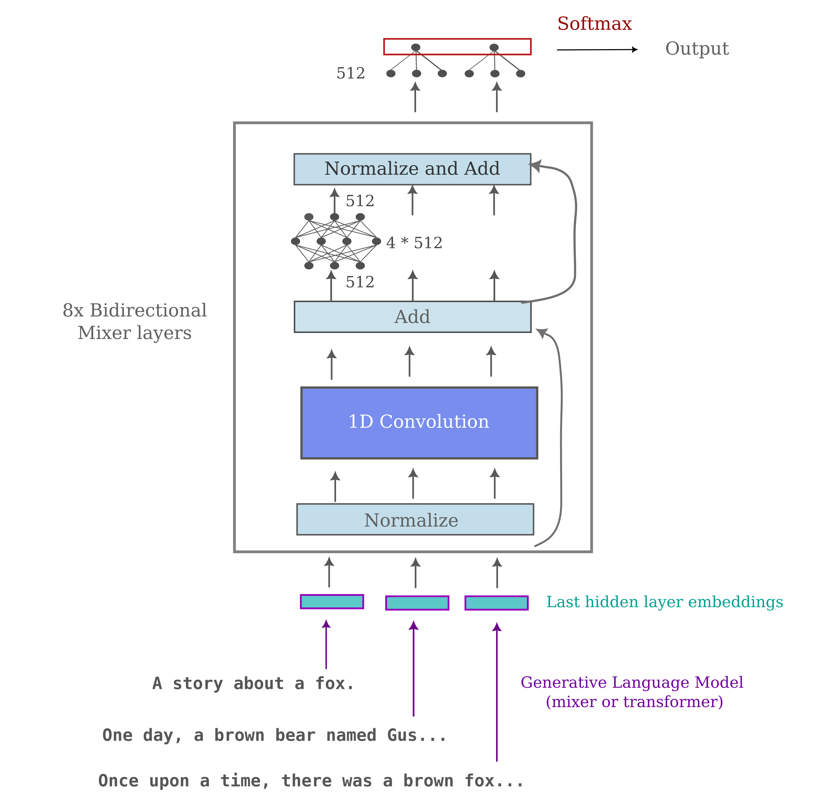
It should be noted that this approach does have practical value: one can perform a B-tree -like algorithm for finding matches from $n$ samples in $n \log n$ forward passes of the sequence matching model.
The retrieval pairs themselves are one-sentence summaries, and were generated for the first 200k tinystories samples by the instruction-tuned version of Llama-3 (8b). We have seen that the embeddings formed by masked mixers contain much more information about the input than those formed by transformers, so the hypothesis is that the retrieval process will be far more successful after identical training runs.
And indeed this is what is found: for 200k summary-story pairs with 32 samples being considered at one time (the ‘context’), the mixer’s embeddings lead to a train/test loss of 0.05/0.29 whereas the transformer of the same output dimension (1024) peaks at 0.01/0.40. When the number of samples increases the gap widens considerably: for a context size of 128, the mixer achieves train/test losses of 0.01/0.76 where the test loss continues to decrease even after 200 epochs, whereas the transformer only manages peak losses of 0.61/2.27 with severe overfitting (the training run ends at 2.98 test loss).
The mixer has another significant advantage with respect to embedding training: with relatively fewer inter-token parameters for a given $d_{model}$ size, the mixer is able to form a more high-dimensional embedding with the same compute resources as a transformer. The effect of this is that the transformer architecture with the lowest loss after the 12-hour 3060 compute on TinyStories ($d_m=512, n_l=8, h=4, \eta=0.005$) yields a 512-dimensional embedding that results in very poor matching model training even for the limited 32 context window size (virtually no train or test loss after 200 epochs at 3.43, whereas an identically-sized masked mixer achieves cross-entropy losses of 0.01 train and 0.10 test.
With an increase in the number of samples available, the mixer is capable of better performance: for the 512-dimensional masked mixer embeddings given a 32-sized comparison batch the test loss decreases from 0.1 to 0.053. As the number of samples increases to 550k, and likewise for a 128-sized batch we have a test loss of 0.12.
It is interesting to note that an untrained mixer, while able to accurately represent its input, yields very poor embeddings for retrieval training. For the 200k dataset, an untrained 512-dimensional masked mixer’s embeddings lead to practically no learning for batches of size 128 and even for batches of size 32 there is severe overfitting, with loss not below 3.2. Even more unexpected is the finding that the last hidden layer embedding is equally poor for retrieval tasks if the embedding model undergoes autoencoding rather than causal language model training (ie next token prediction). This can be shown by training an encoder-decoder architecture where the encoder mixer’s last token’s last hidden layer embedding is repeated to a decoder, which is tasked with regenerating the entire input string. This encoder-decoder may be trained remarkably effectively (with <2.0 cross-entropy loss) but the encoder’s embedding is no better than that from an untrained model for retrieval learning. This suggests that the causal language model training process itself is important to language retrieval.
It may be wondered if this is a result of some kind of incompatibility between a transformer’s embedding and the ability of a mixer to learn that model’s manifold, but this is not the case: if we instead use a bidirectional transformer to learn the retrieval pairs from the transformer’s embeddings, we find that this model is far worse than the bidirectional mixer and that practically no learning occurs.
Thus we find that for embedding models of various sizes, embeddings derived from masked mixers lead to far better performance on a retrieval training task when compared to transformers. This supports the hypothesis that the full sequence-to-sequence mapping that is performed during retrieval benefits greatly from the increased informational content in the masked mixer’s embedding as compared to the transformer’s.
Conclusions
Seeking to make a more efficient learning algorithm than a transformer, we used the observation that input representation is far superior for modified MLP-Mixer architectures to craft a model capable of replicating the autoregressive language generation of GPT-style decoder-only transformers.
We have seen that masked mixers are typically more efficient learners than transformers for the task of causal language modeling on TinyStories with no changes to the default architecture. Mixers are typically competetive with or slightly wores than hyperparameter-optimized transformers on newer hardware with key, query, and value optimizations like Flash Attention 2, depending on the hardware. Masked mixers are, as implemeted, less efficient for CLM inference because they are highly parallelized and have a fixed-size context window for each forward pass.
On the other hand, masked mixers as they exist today are far more effective at retrieval tasks as evidenced by the observation that a summary-story matching retrieval model is capable of far better training on embeddings from these models compared to embeddings from transformers. For this task, inference would be approximately identical as one typically loads full context for each forward pass for retrieval tasks.
It is worth restating the more noteworthy findings of this work concisely:
- Depending on the hardware the models are implemented on, given equal compute a masked mixer may reach a much lower training and validation causal language model loss or else a modern, dataset-optimized transformer may out-perform the mixer.
- The mixer implementations uses no traditional regularization techniques, instead relying on the intrinsic generalization inherent in gradient descent-based optimization of high-dimensional space (see this paper for more on this subject) combined with the ‘inherent’ regularization in language datasets. Mixers also have no rotary positional encoding (or any explicit positional encoding at all). Positional encoding instead stems directly from the convolutional filter weights.
- Compared to the transformer models as originally introduced or adapted for CLM, masked mixers are more efficient learning algorithms. It is only with the optimizations of recent years (RoPE, FA2 etc) that the transformer becomes competitive for causal language modeling.
- As mixers exhibit far more accurate input representations and thus contain more information on the input than transformers, one expects better sequence-to-sequence retrieval performance from these models. This is experimentally supported when training a retrieval model on mixer or transformer embeddings.
Fundamentally the masked mixer may be thought of as a true feedforward model in which all elements of the input are processed in parallel by sequential models. Transformers on the other hand are conceptually somewhat parallelized (as otherwize the causal language mask training trick would not work) but still retain aspects of recurrent neural networks (backpropegation must unroll the KV values, for example) which makes them faster for inference but slower to train. When one considers that training a language model may require a trillion times more compute than autoregressive inference, this shift does not seem to be entirely uncalled for. For retrieval tasks this does not apply, as the models are typically applied to chunks of data at fixed input sizes.
To conclude, the masked mixer architecture is introduced, motivated by superior input representation accuracy in this model compared to the transformer. This mixer architecture is in many ways much simpler than the transformer, but performs suprisingly well considering the many optimizations introduced since the first transformer architecture in 2017. Transformer-mixer hybrids offer the most efficient models observed for this dataset, outperforming Llama style models with many of the latest optimizations (Flash attention 2, RoPE etc.). These results indicate that a highly optimized transformer with its intrinsic focus on relatively few input elements for each output results in approximately as or slightly more efficient a learning paradigm as the masked mixer’s lack of focus if the transformer is properly tuned, depending on the hardware.
Returning to our original question: how many parameters are necessary for effective language modeling? We hypothesized that a masked mixer with (much) better representational accuracy than the transformer would outperform that model in causal language modeling tasks given a fixed amount of compute, but found that although a naieve implementation of each model did result in much better performance from the masked mixer, a combination of architectural, implementation, and hyperparameter optimizations allows the transformer to learn approximately as efficiently as or slightly better than the mixer depending on the hardware. On the other hand the masked mixer far outperforms the transformer for tasks involving matching one sequence of words to another, suggesting that representational accuracy is indeed important for that task.
How many parameters are required for accurate modeling of the TinyStories, at least the train split of that dataset? We can estimate this as follows: in our (slightly truncated training) dataset there are 2M stories, and each story is composed of perhaps 256 tokens for a total of 512M tokens. Assuming that training proceeds via next token prediction, this means that there are 512M ‘next’ tokens and thus 512M points that must be approximated in high-dimensional space. From the Johnson-Lindenstrauss lemma we can estimate that this would require an embedding space $n$ such that
\[n > 8 \ln (512 \times 10^6) \approx 160\]If we assume that each model layer’s $d_{model}$ corresponds to the model’s dimension, this means that even the smaller mixers should be able to effectively memorize the entirety of the training portion of TinyStories. This is somewhat well-supported in our experimental results, as 512 or 1024-dimensional models were apparently capable of reasonably low cross-entropy loss even given very limited compute.
On the other hand, if it is more accurate to assume that each of the model’s parameters corresponds to a dimension then even the smallest model we used should have no trouble memorizing TinyStories, which is not observed. This means that the former picture of model dimensionality seems more accurate experimentally, and this is supported by other work which finds that a model’s parameters from one layer to the next certainly do not vary independently, and therefore may not be considered to be uniqe dimensions in high-dimensional space.