Autoencoders: Learning by Copying

Introduction

Autoencoders are machine learning models that attempt to replicate the input in their output. This endeavor may not seem to be very useful for tasks such as generating images or learning how inputs are related to one another, particularly when the models used are very large and fully capable of learning the identity function on the input. Indeed, in the past it was assumed that models capable of learning the identity function (typically models with more neurons per layer than input elements) would do so without other forms of regularization.

Historically, therefore, autoencoders were studied in two contexts: as undercomplete models that compressed the input in some useful way, and as possibly overcomplete models that were subject to certain restrictions to as to prevent the learning of the identity function. Here ‘overcomplete’ is used more informally than the strict linear algebra term, and signifies a model that has more than enough elements (neurons) per layer to exactly copy the input onto that layer.

A number of useful models have resulted from those efforts, including the contractive autoencoder which places a penalty on the norm of the Jacobian of the encoder with respect to the input, and the variational autoencoder which simultaneously seeks to minimize the difference between autoencoder output and input together with the difference between the hidden layer code $z$ given model inputs and a Gaussian distribution $N(z; I)$.

The primary drawback of these regularized autoencoders is that they tend to be incapable of modeling the distribution of inputs given to the model to a sufficient degree, which manifests experimentally as blurriness in samples drawn from these models. For variational autoencoders, there is a clear reason why samples would be blurry: transforming a typical image using a Gaussian distribution (via convolution or a similar method) results in a blurry copy of that image, so it is little surprise that enforcing the encoding of an input to approximate a Gaussian distribution would have the same effect. As a consequence of this challenge, much research on generative models (particularly for images) has shifted away to generative adversarial networks and more recently diffusion models.

Recently, however, two findings have brought the original assumption that overcomplete autoencoders would memorize their inputs into question. First, it has been observed that deep learning models for image classification tend to lose a substantial amount of input information by the time the input has been passed to deep layers, and that trained models learn to infer this lost information (reference). Second it has been found that image classification models are more or less guaranteed to generalize to some extent when trained using gradient descent (reference).

In light of these findings, it is worth asking whether overcomplete deep learning autoencoders will necessarily memorize their inputs. The answer to this question is straightforward, as we will see in the next section.

Overcomplete autoencoders do not learn the identity function

The question of whether overcomplete autoencoders memorize their inputs can easily be tested by first training an autoencoder to replicate inputs, and then observing the tendancy of that autoencoder to copy its inputs after small changes are made. Autoencoders may be trained in various ways, and we choose to employ the minimization of Mean-Squared Error between the input $a$ and reconstructed input $D(E(a))$ where $D$ signifies the decoder of hidden code $h$, $E$ the encoder which maps $a \to h$ and $O(a, \theta)$ the output of the encoder and decoder given model parameters $\theta$.

\[L(O(a, \theta), a) = || D(E(a)) - a ||^2_2\]

Mean-squared error loss in this case is equivalent to the cross entropy between the model’s outputs and a Gaussian mixture model of those outputs. More precisely assuming that the distribution of targets $y$ given inputs $a$ is Gaussian, the likelihood of $y$ given input $a$ is

\[p(y | a) = \mathcal{N}(y; \mu (O(a, \theta)), \sigma)\]

where $\mu (O(a, \theta))$ signifies the mean of the output and $y=a$ for an autoencoder.

As for the case observed with variational autoencoders, it has been assumed that training autoencoders via MSE loss results in blurry output images because it implies that the input can be modelled by a Gaussian mixture model. And for a sufficiently small model this is true, being that only a small number of Gaussian distributions may compose the mixture model.

But for a very large model it is not the case that MSE loss (or any maximum likelihood estimation approach) will necessarily yield blurry outputs because the Gaussian mixture model is a universal approximator of computable functions if given enough individual Gaussian distributions independent from each other given weights $w_1, w_2, … w_n$

\[g(a; w, \mu, \sigma) = \sum_i w_i \mathcal{N}(a; \mu_i, \sigma_i)\]

Therefore it can be theoretically guaranteed that a sufficiently large autoencoder trained using MSE loss on the output alone will be capable of arbitrarily good approximations on a given input $a$ (and will not yield blurry samples).

This being the case, we can now test whether an overcomplete autoencoder trained using gradient descent to minimize MSE loss will memorize their inputs. Memorization in this case is equivalent to learning the identity function, so we can test memorization by simply changing an input some small amount before observing the output. If the identity function has been learned then the model will simply yield the same input back again.

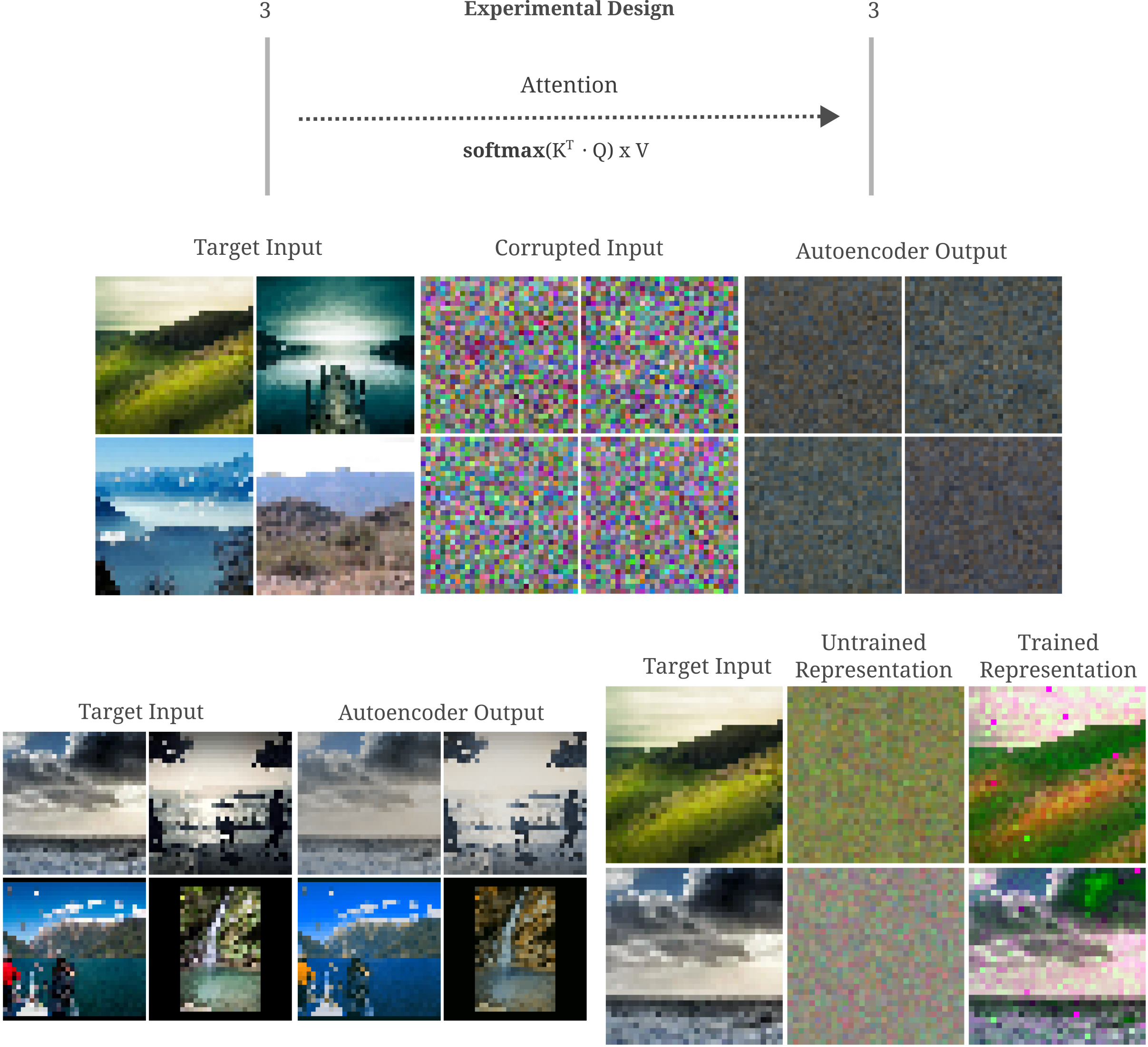
One such change to an input is the addition of noise. In the following experiment we train a 5-hidden layer feedforward model, each layer having more elements that the input. As shown in the figure below, we find that indeed the overcomplete autoencoder does not memorize its inputs: upon the addition of Gaussian noise $\mathcal N(a \in [0, 1]; \mu=7/10, \sigma=2/10)$

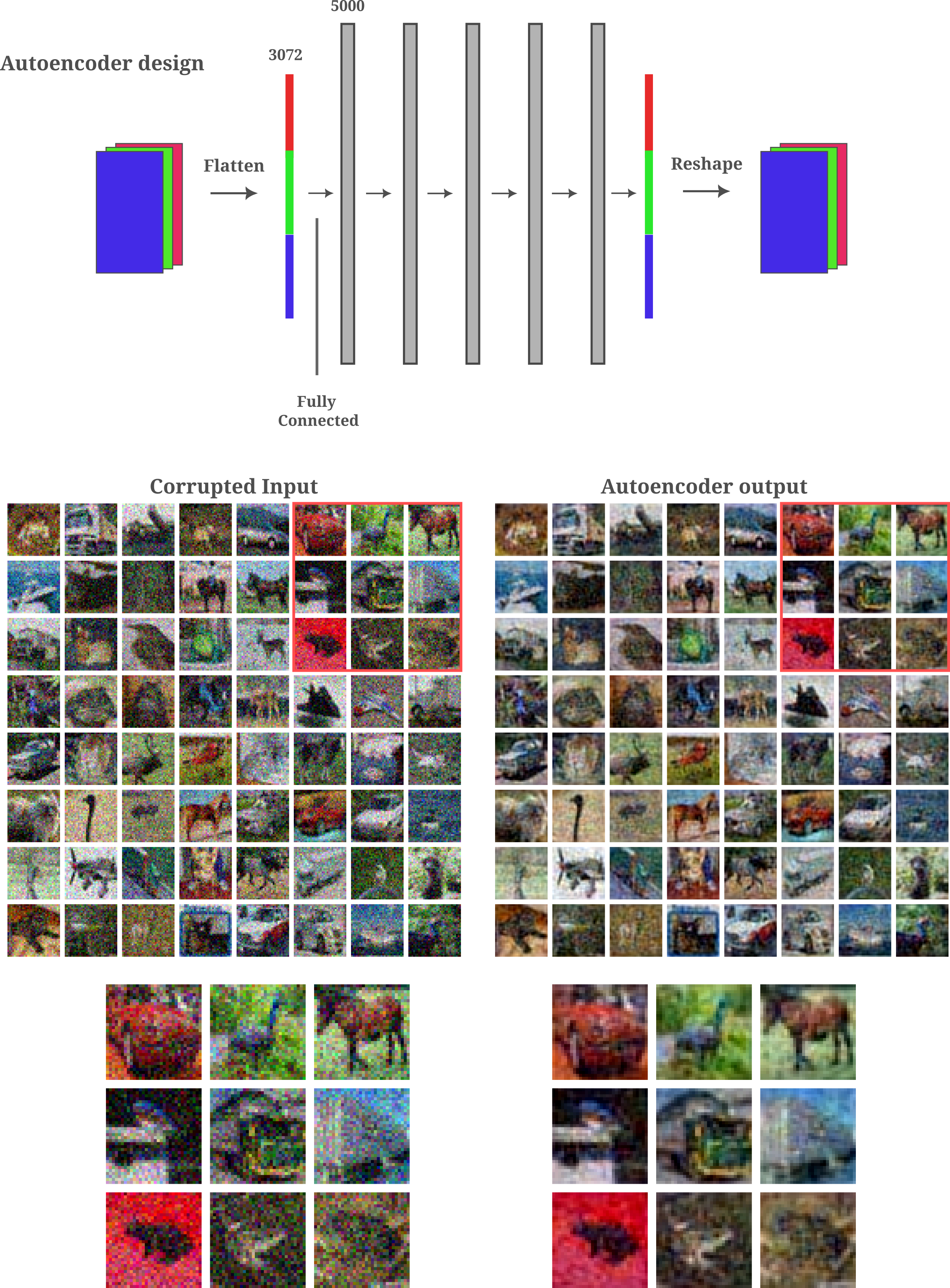
This experiment provides evidence for two ideas: first that overcomplete autoencoders do not tend to learn the identity function as evidenced by the difference in the autoencoder’s output given a noise-corrupted input, $O(\widehat a, \theta)$ compared to the original input $a$, and second that the output actually de-noises the input such that

\[||O(\widehat a, \theta) - a|| < || \widehat a - a ||\]

The latter observation is far from trivial: there is no guarantee that a function learned by an autoencoder, even if this function is not the identity, would be capable of de-noising an input. We next investigate why this would occur.

Autoencoders are capable of denoising without being trained to do so

To re-iterate, elsewhere it was found that deep learning models lose a substantial amount of information about the input by the time the forward pass reaches deeper layers, and furthermore that moels tend to learn to infer that lost information upon training. The learning process results in arbitrary inputs being mapped to the learned manifold, which for datasets of natural images should not normally be approximated by Gaussian noise. The learning process for natural image classifiers is therefore observed empirically to be as analagous to learning how to de-noise an input. One may safely assume that the same de-noising would occur upon training an autoencoder.

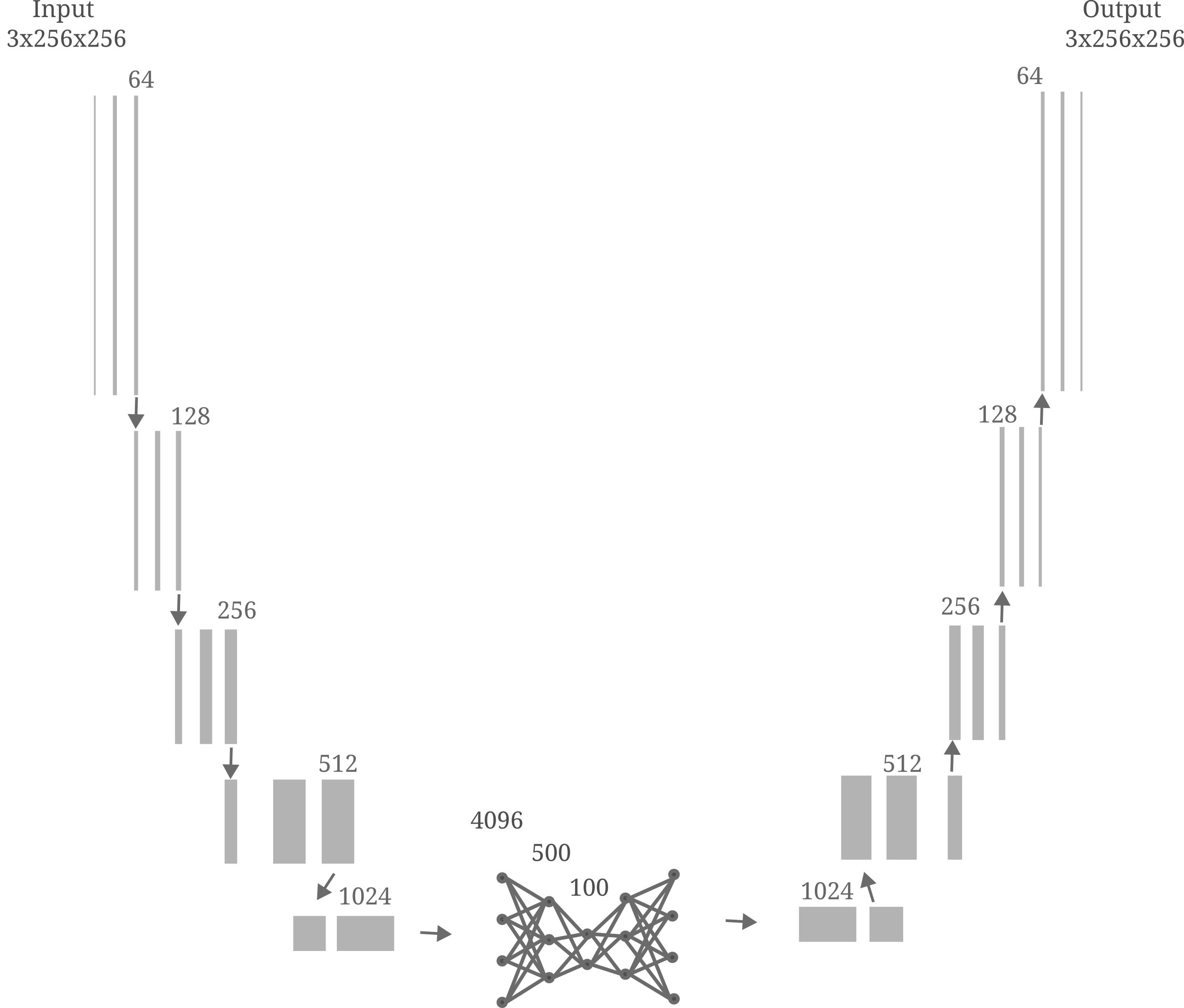
For this section and much of the rest of this page, we will employ a more sophistocated autoencoder than the one used above. We use U-net, a model introduced by Ronneburger and colleagues for medical image segmentation.

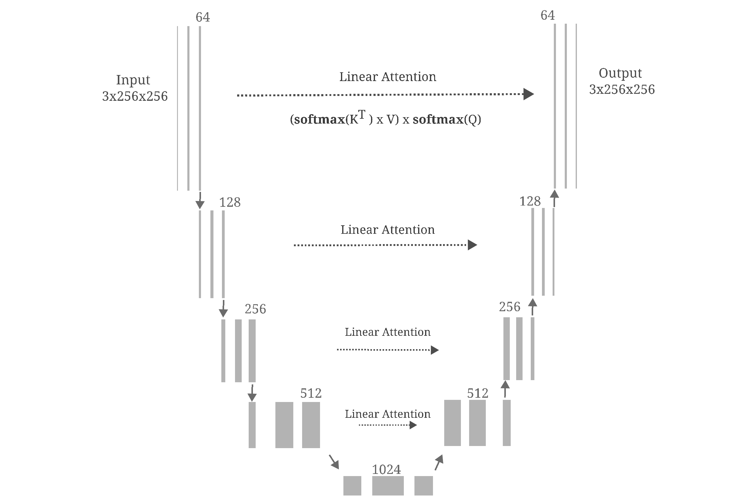
The U-net was named after it’s distinctive architecture, which can be visualized as follows:

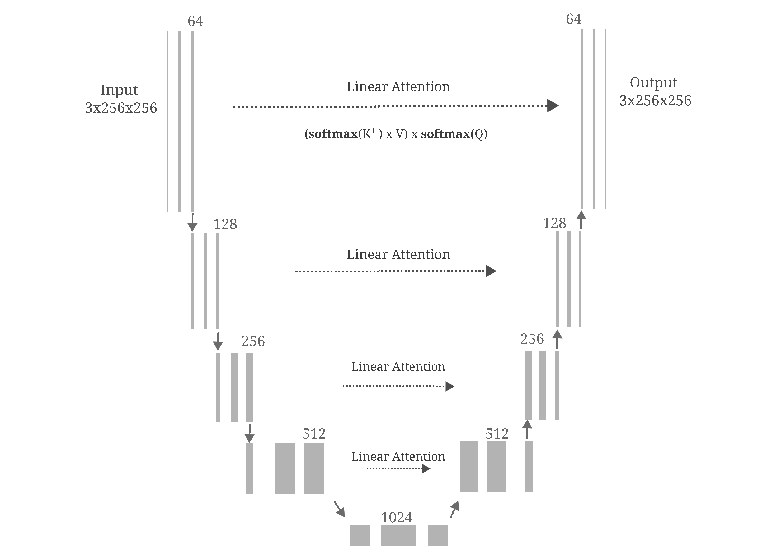
For now, we make a few small adjustments to the Unet model: first we remove residual connections (which if not removed do lead to a model learning the identity function because it is effectively low-dimensional) and then we modify the stride of the upsampling convolutions to allow for increased resolution (code is available here). Notably we perform both training and sampling without switching to evaluation mode, such that the batch normalization transformations do not switch the batch’s statistics with averages accumulated during training.

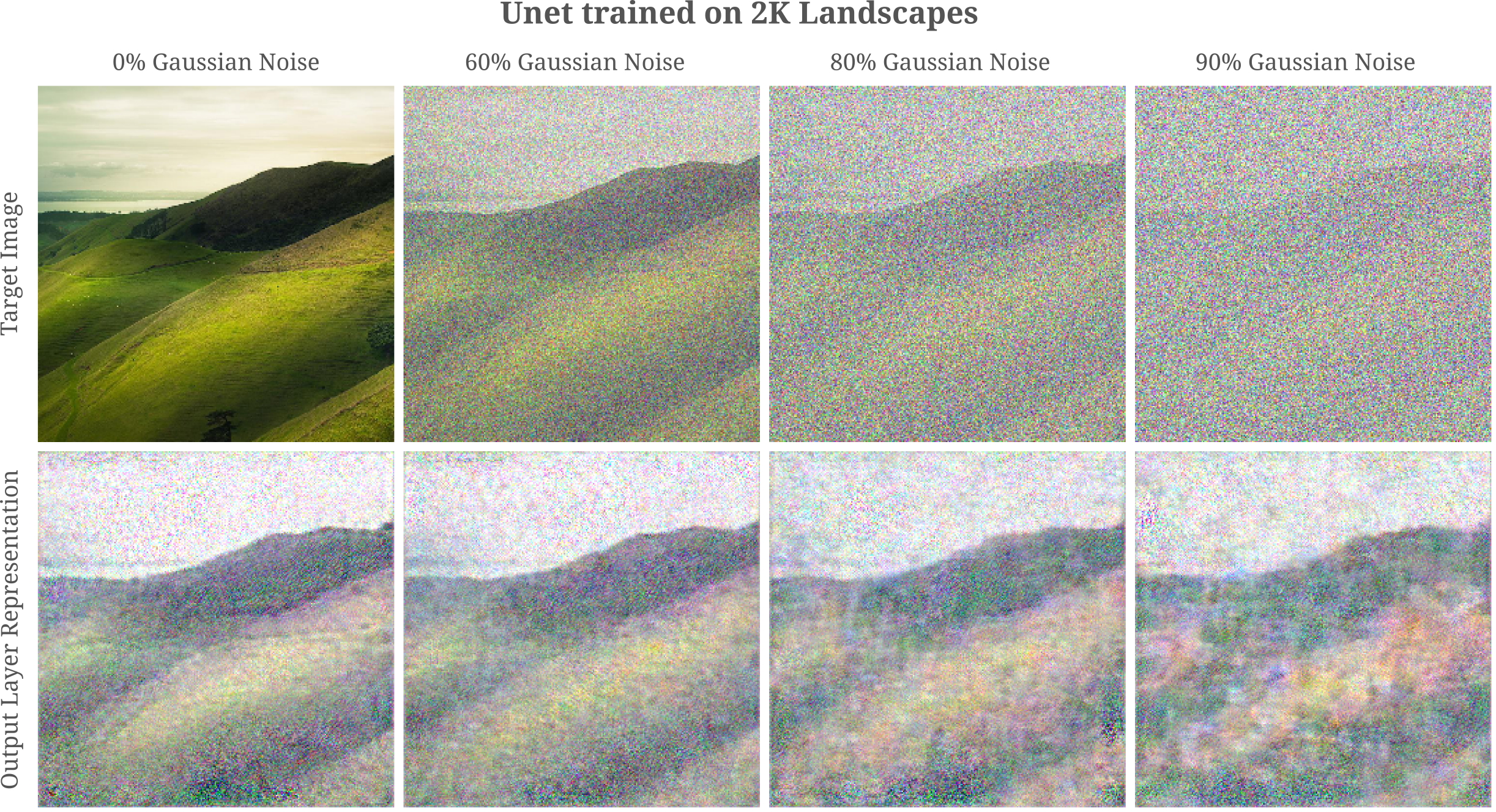
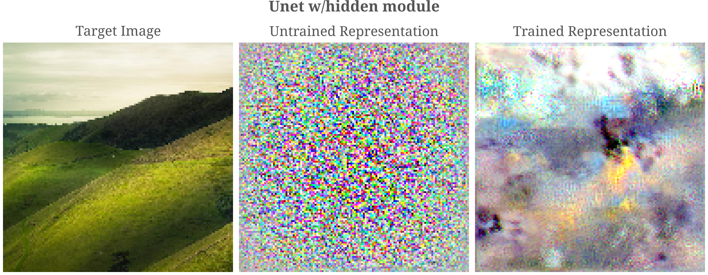
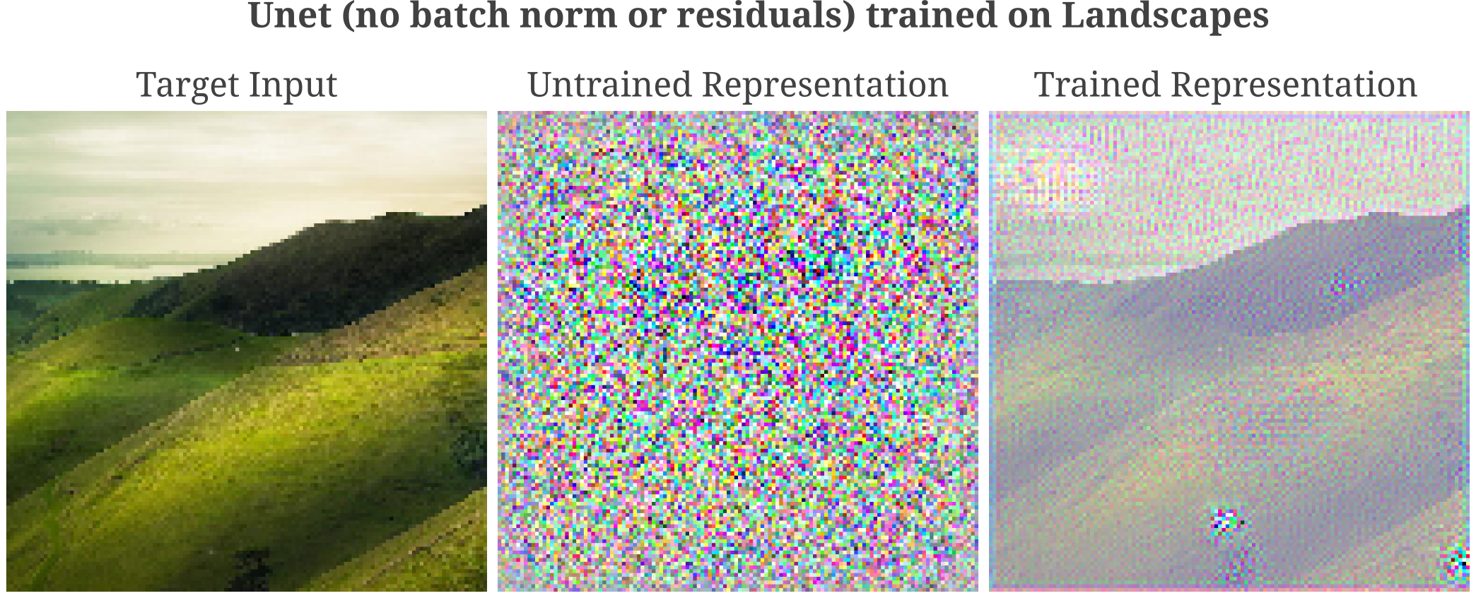
Returning to the question of the tendancy of training to reduce noise in an autoencoder, take the last layer’s representations of the input in trained versus untrained Unet model (without residual layers) shown in the following figure.

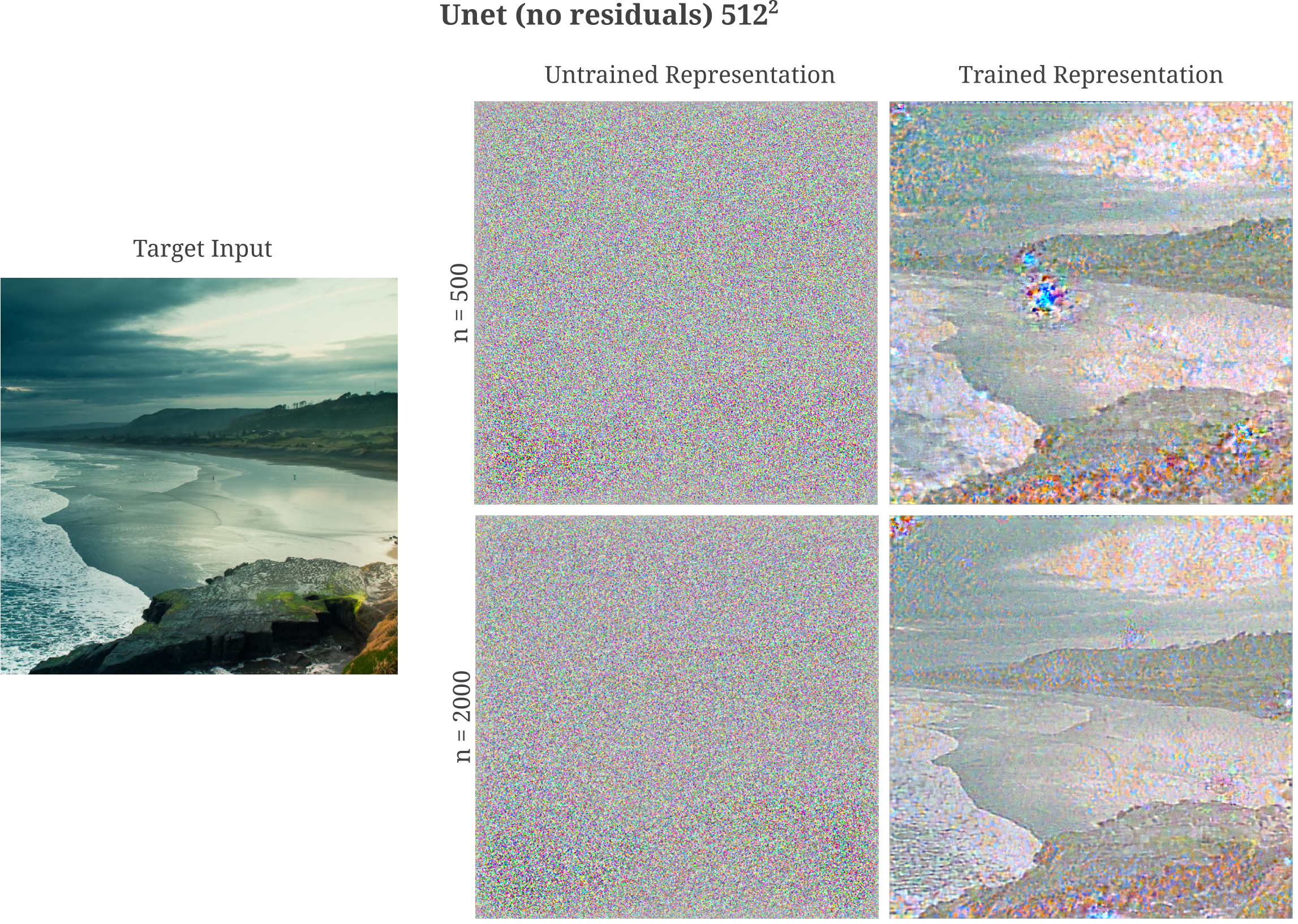
The trained model has clearly learned to reduce the noise in the last layer’s representation relative to the untrained model. It may thus be wondered whether autoencoders are capable of learning to de-noise inputs.

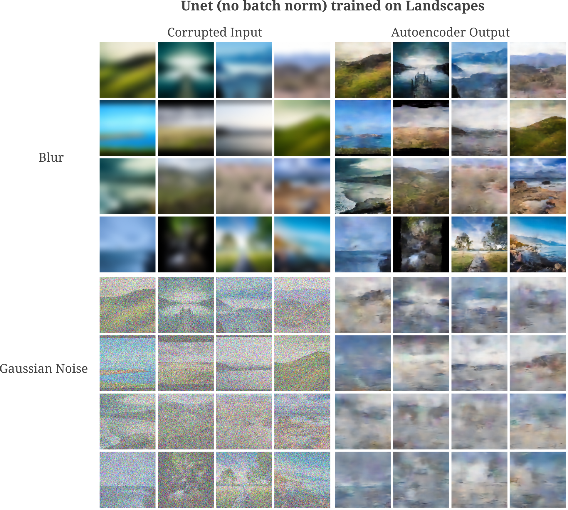
The same ability of autoencoders to de-noise is observed for Unet applied as an autoencoder for lower-resolution images, here 64x64 LSUN church images.

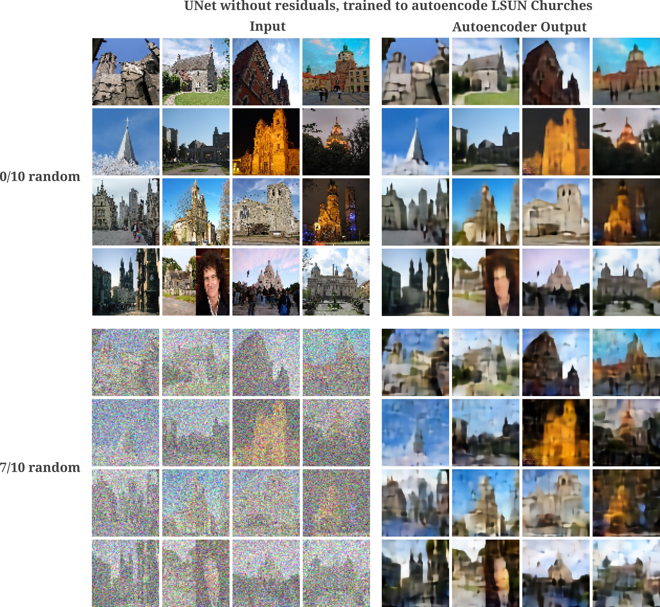
With more training, we see that images may be generated even with a large addition of noise

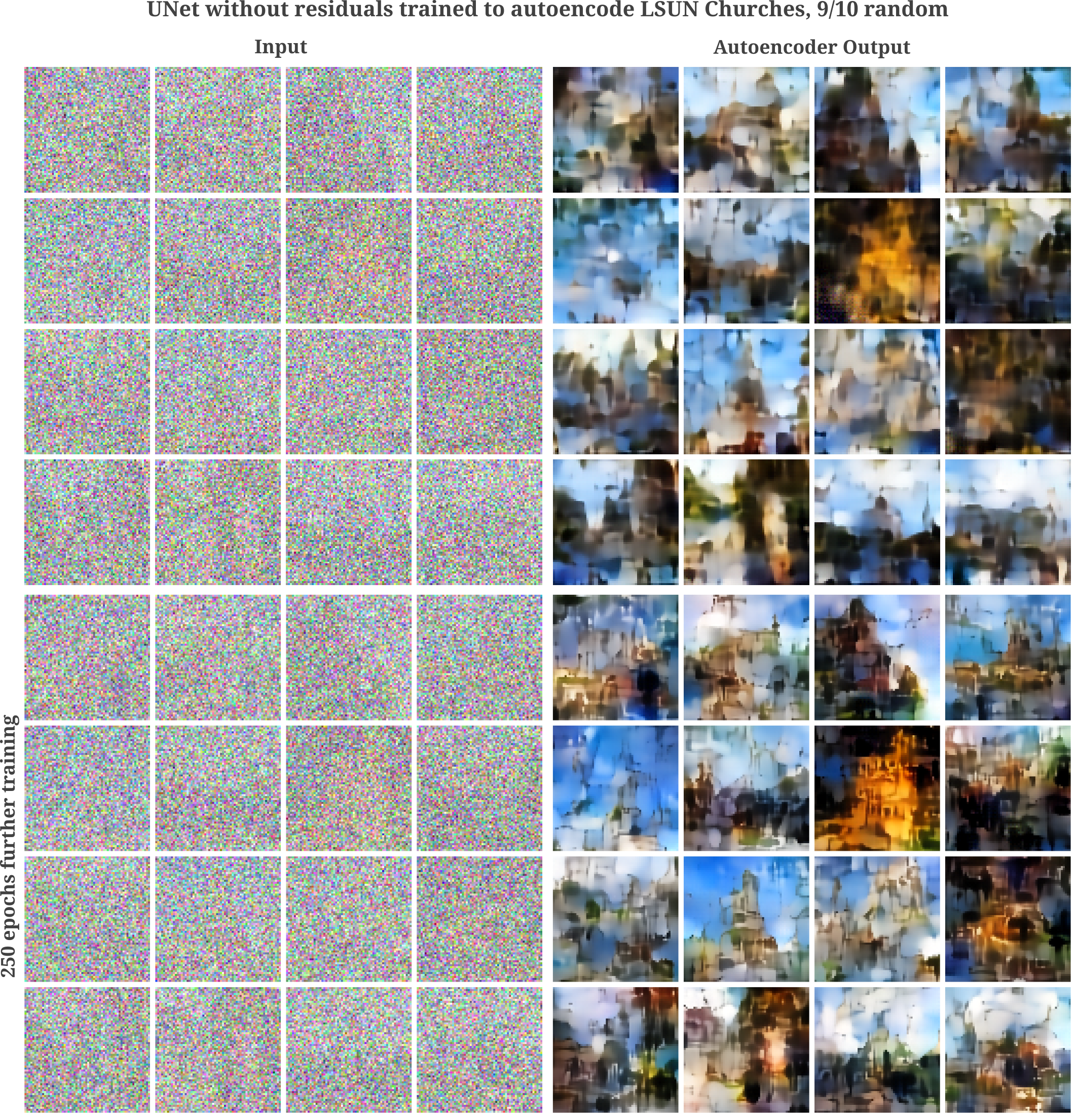
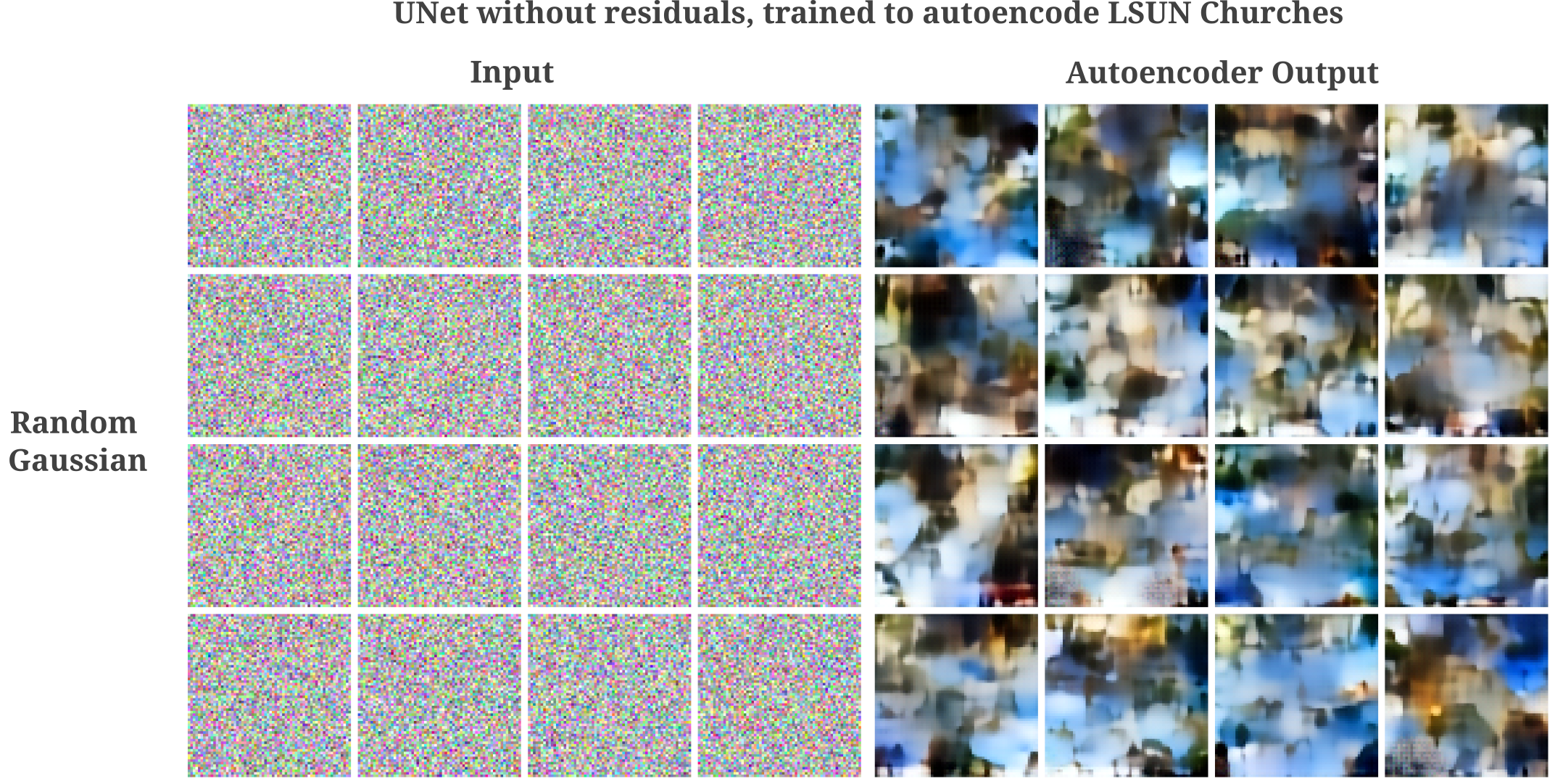
and for pure noise, we have the following:

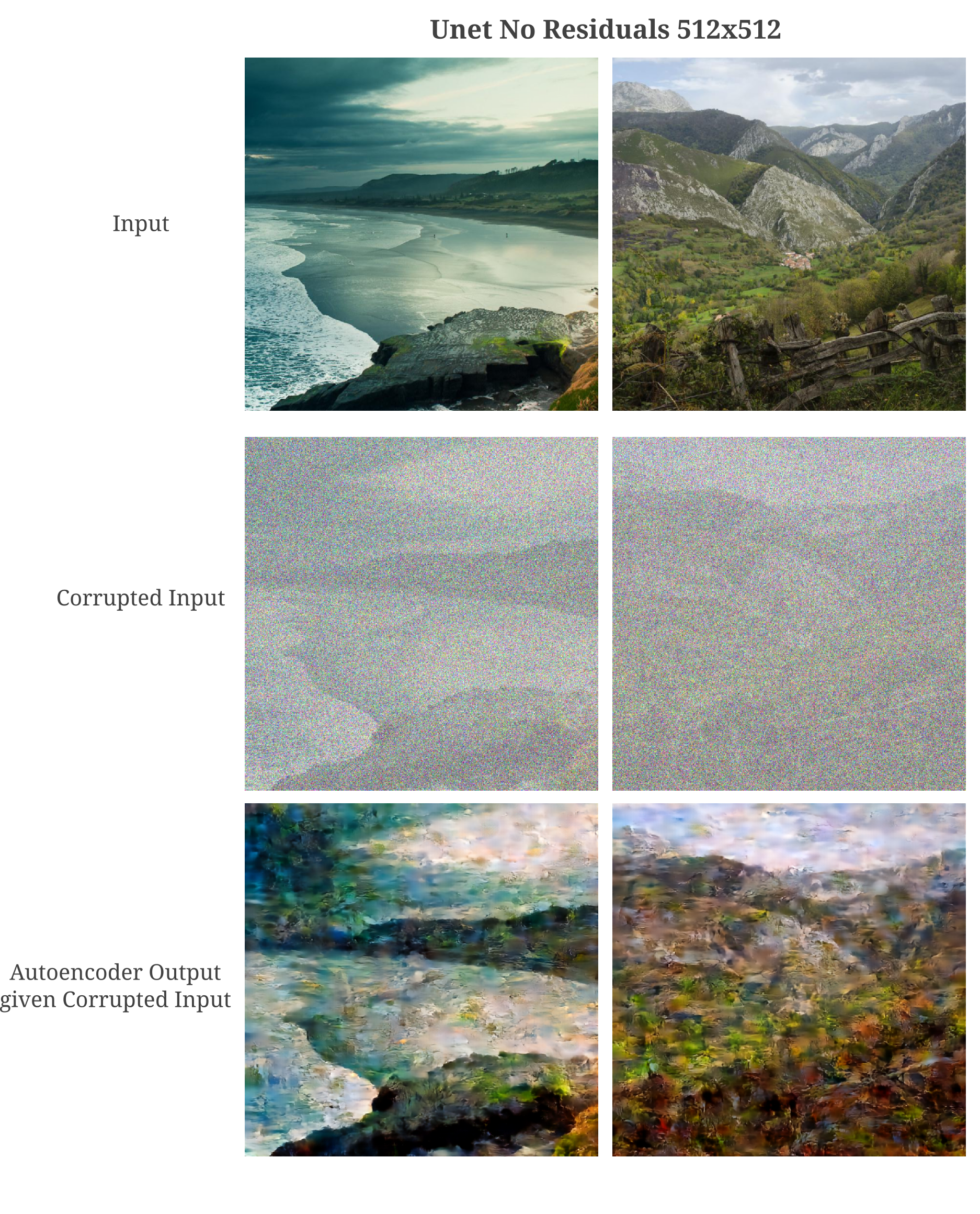
Early in this section we have seen that autoencoder training leads to the de-noising of Unet’s representation (in the output layer) of its input. After we have seen how Unet is capable of an extraordinary amount of denoising even without being trained to do so. It may be wondered if these two phenomena are connected, that is, if denoising occurs because the learned representation has less noise than the input. If this were the case then we would expect a noise-corrupted input to lose some of this noise not only in the autoencoder output but also in the autoencoder’s output layer representation of its input. Our expectation is correct, as we can see in the following figure:

It may be wondered then if there is necessarily an equivalence relation between the ability of an autoencoder to accurately represent its input (and hence to de-noise the original representation as we will see in the next section) and the ability to accurately autoencode. The answer here is no, not necessarily: given a powerful enough decoder, most information from the input can be lost and an accurate encoding can be made. For example, if a restrictive three-hidden-layer module is inserted into the Unet (see later sections for more details) then the model is capable of accurate autoencoding (and substantial de-noising) but does not accurately represent its input as shown in the following figure.

Why Noninvertibility introduces Gaussian Noise in Input Representations

So far we have seen empirically that autoencoders are capable of removing noise from an input even when they are not explicitly trained to do so. This may be understood to be equivalent to the finding that autoencoders learn manifolds that are not noisy, and map arbitrary inputs (even noisy ones) to that manifold.

There is another related phenomenon that may also play a role in the ability of autoencoders to denoise: the non-invertibility of transformations in untrained models introduces noise into the representations of the input, but much of this noise is removed from the representation during the training process. Noise is introduced between non-invertible (or approximately non-invertible) transformation representations because many possible inputs may yield one identical output for models composed of non-invertible (singular) linear transformations. These many possible inputs closely resemble Gaussian noise if the models in question are composed of transformations that are independent which is indeed the case for typical deep learning models at initialization.

To be precise, suppose we are given a simple fully connected model that has been initialized with weights initialized to a uniform distribution, $w_n \sim \mathcal U$ (which is the default for Pytorch). For the purposes of this argument, these weights could actually be distributed in any number of ways so long as the initialization is random and does not vary too much between layers.

First assume that an input to be transformed into a representation $x_i$ is initialized near the origin, perhaps to uniform values. Now suppose that the model were composed of one or more layers, each layer being a linear transformation (matrix multiplication) $A_l$ from dimension $n \to m: n > m$ such that the output dimension $d$ is much smaller than the input dimension $D$. The representation of the output $O(a, \theta)$ by the input is defined as an input $x_i$ such that $O(x_i, \theta) = O(a, \theta)$. We can show here that given these assumptions the input representation is approximately normal before training, or $O(x_i, \theta) \sim \mathcal N$.

To see this, first take a model composed of a single linear transformation. Assuming full rank for $A_1$, the number of dimensions in which $x_n$ can change is $n - m$. For large $n$, the chance that an element of $x_i > \epsilon$ is equal to the volume of a point in an n-dimensional sphere greater than $\epsilon$ away from the origin, which is equal to

\[vol(d) \leq 2 \mathrm{exp} (-n \epsilon^2 / 4) v_n\]

whereas the probability for a point in the normal distribution to exceed $\epsilon$ away from the expectation is

\[p(|x-\mu| > \epsilon) = \mathrm{exp}(-2n\epsilon^2)\]

This is for one layer: for $k$ layers in a model, the number of dimensions in which $x_n$ has freedom to change is $(n_1 - m_1) (n_2 - m_2) \cdots (n_k - m_k)$.

It may be wondered why trained models then do not typically have representations that resemble Gaussian noise. The answer is that after training we can no longer assume that sucessive layers contain weights that are independent: to put it concretely, the linear combinations of successive layers are no longer guaranteed to be orthogonal such that the representation of an output layer in a deep model is lower-dimensional than that of an untrained model.

But notably even trained models would be expected to have Gaussian noise-like corruption after one or a few non-invertible layers, if those layers were composed of non-invertible transformations $n \to m: m « n$. This is because the dimensions in which an input of a linear transformation with $n > m$ may vary for some fixed $f(x) = y$ are necessarily orthogonal, which is a result of the fundamental theorem of linear algebra. Assuming that the orthogonal dimension number $m - n$ is sufficiently large, a point chosen near the origin from these dimensions is approximately Gaussian as shown above.

This theory is supported by experimental evidence: observe that for vision transformers the representation of block 1 (which has only two fully connected layers per patch, ignoring attention transformations between patches) for trained and untrained models alike contains noticeable Gaussian noise whereas the deep layers of untrained but not trained models exhibits any Gaussian noise. This is precisely what the theory predicts if training removes independence of weights from one layer to the next.

Image Generation with an Autoencoder Manifold Walk

Earlier on this page we have seen that even very large and overcomplete autoencoders do not learn the identity function but instead capture useful features of the distribution of inputs $p(a)$. We were motivated to investigate this question by the earlier findings that deep learning classification models tend to generalize even when they are capable of memorization, and that deep layers are typically incapable of exactly representing the input due to approximate and exact non-invertibility.

We can postulate that the theory behind generalization of classifiers also applies to autoencoders as long as they are trained using gradient descent, as there is no stipulation in the original work that the dimensionality of the output is less than the input, or that the models must be trained as classifiers (ie with one-element $\widehat y$ target values).

Likewise, it seems fairly obvious that an inability of a deep layer (which could be an autoencoder output) to represent the input at the start of training would also prevent memorization to some extent, being that it would be highly unlikely for a model to learn the identity function if deeper layers cannot ‘know’ exactly what the input looks like.

We next saw how autoencoders are effective de-noisers, and that at the start of training typical deep learning archictures induce Gaussian noise in subsequent layers such that the model must learn to reduce such internal noise during training. Being that there is no intrinsic difference between internal and input-supplied Gaussian noise, it is not particularly surprising that sufficiently deep autoencoders are capable of powerful noise reduction.

This being the case, it should be possible to generate inputs from the learned distribution $A \sim \widehat{p}(a)$ assuming that the learned distribution approximates the ‘true’ data distribution, ie $\widehat{p}(a) \approx p(a)$.

For overcomplete autoencoders, however, we are presented with a challenge: how do we navigate the latent space to synthesize a sample, given that for a high-dimensional latent space may be large such that only a small subregion of this space is actually explored by the model’s samples? For example, say the dimensionality of the smallest hidden layer of the autoencoder (which we take to be the latent space) is larger than the dimensionality of the input. Simply assigning the values of this latent space as a random normal distribution before forward propegating this information to the output is not likely to yield an image representative of $p(a)$ unless samples of $p(a)$ yielded a similar distribution in that latent space.

This is extremely unlikely unless some constraints are placed on the model, and indeed a very similar model to the one we have considered here has been investigated. These models are called variational autoencoders, and although effective in many aspects of probability distribution modeling they suffer from an inability to synthesize sharp images $A$, which can be attributed to the restrictive nature of mandating that the latent space be normally distributed.

Instead of enforcing restrictions on our model, we can instead map inputs to the learned manifold and perform a walk on this manifold, effectively creating a Markov process to generate images. Suppose we split the Unet autoencoder into two parts, an encoder $\mathcal E$ that takes inputs $a$ and yields a hidden space vector $h$ along with a decoder $\mathcal D$ that takes as an argument the hidden space vector $h$ and yields the synthesized image $g$

\[g = \mathcal D(\mathcal E(a)) = \mathcal D(h)\]

Being that $h$ is not low-dimensional but $\mathcal D(\mathcal E(a))$ has learned $p(a)$, we can first find the hidden space vector $h$ corresponding to some set of $A \sim p(a)$

\[h_1' = \mathcal E(a)\]

Adding a small amount of normally distributed noise to this latent space gives a new latent space point

\[h_1 = h_1' + \mathcal N(h_1'; 0, \epsilon)\]

Then using this latent space vector the corresponding synthesized images are

\[g_1 = \mathcal D(h_1)\]

Now $g_1$ is likely to be extremely similar or identical to $a$ as long as the learned manifold is not too unstable. But if we then repeat this procedure many times such that the Markov chain may be expressed as

\[h_{n+1}' = \mathcal E(g_n) \\ h_{n+1} = h_{n+1}' + \mathcal N(h_n'; 0, \epsilon) \\ g_{n+1} = \mathcal D(h_{n+1})\]

we find that the latent space is effectively explored. For a Unet trained on 256 $512^2$ resolution images of landscapes, we have the following over 300 steps on a manifold walk:

Training a generative model on such a small number of images is not likely to yield very realistic inputs, and it appears that the images generated during the manifold walk are locally realistic but globally somewhat incoherent (observe how portions of sky and land tend to pop up over the entire image).

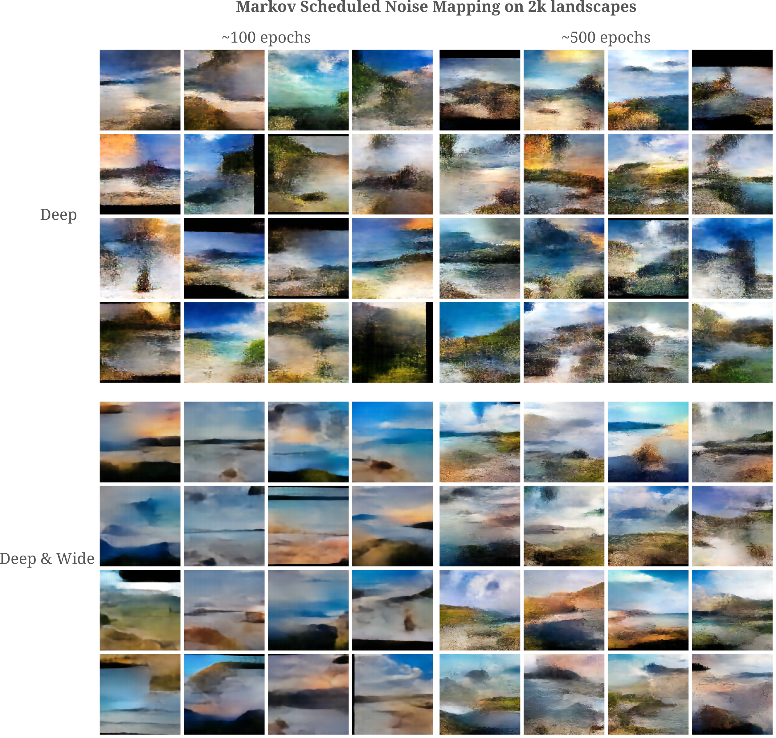
Increasing the dataset size from 256 to 2048 (and decreasing the resolution to $256^2$) we have much more coherent generated images. It is also interesting to note that we see movement between images learned from the training dataset, which is not surprising given that these are expected to exit on the learned manifold.

It is more curious that we see a qualitatively similar manifold even without the addition of noise at each step of the Markov process. More precisely, if we perform the manifold walk as follows

\[h_{n+1} = \mathcal E(g_n) \\ g_{n+1} = \mathcal D(h_{n+1})\]

we find

This shows us that much of the tendancy of repeated mapping to a manifold to lead to movement along that manifold occurs in party due to that manifold’s instability. We can pfind further evidence that most of the manifold walking ability is due to the manifold’s instability by performing the same noise-less Markov procedure on autoencoders after varying amounts of training. With increased training, the proportion of inputs that walk when repeatedly mapped to a manifold decreases substantially: with 200 further epochs, we find that this proportion lowers from 7/8 to around 1/8.

Diffusion with no Diffusion

Given that autoencoders are effective de-noisers, we can try to generate inputs using a procedure somewhat similar to that recently applied for diffusion inversion. The theory here is as follows: an autoencoder can remove most noise from an input, but cannot generate a realistic input from pure noise. But if we repeatedly de-noise an input that is also repeatedly corrupted, an autoencoder may be capable of approximating a realistic image.

To begin, we use a random Gassian distribution in the shape of our desired input $a_g$

\[a_0 = \mathcal N(a; \mu, \sigma)\]

where $\sigma$ and $\mu$ are chosen somewhat arbitrarily to be $7/10, 2/10$ respectively. Now we repeatedly de-noise using our autoencoder but on a schedule: as the number of iterations increases to the final iteration $N$, the constant $c$ increases whereas the constant $d$ decreases commensurately.

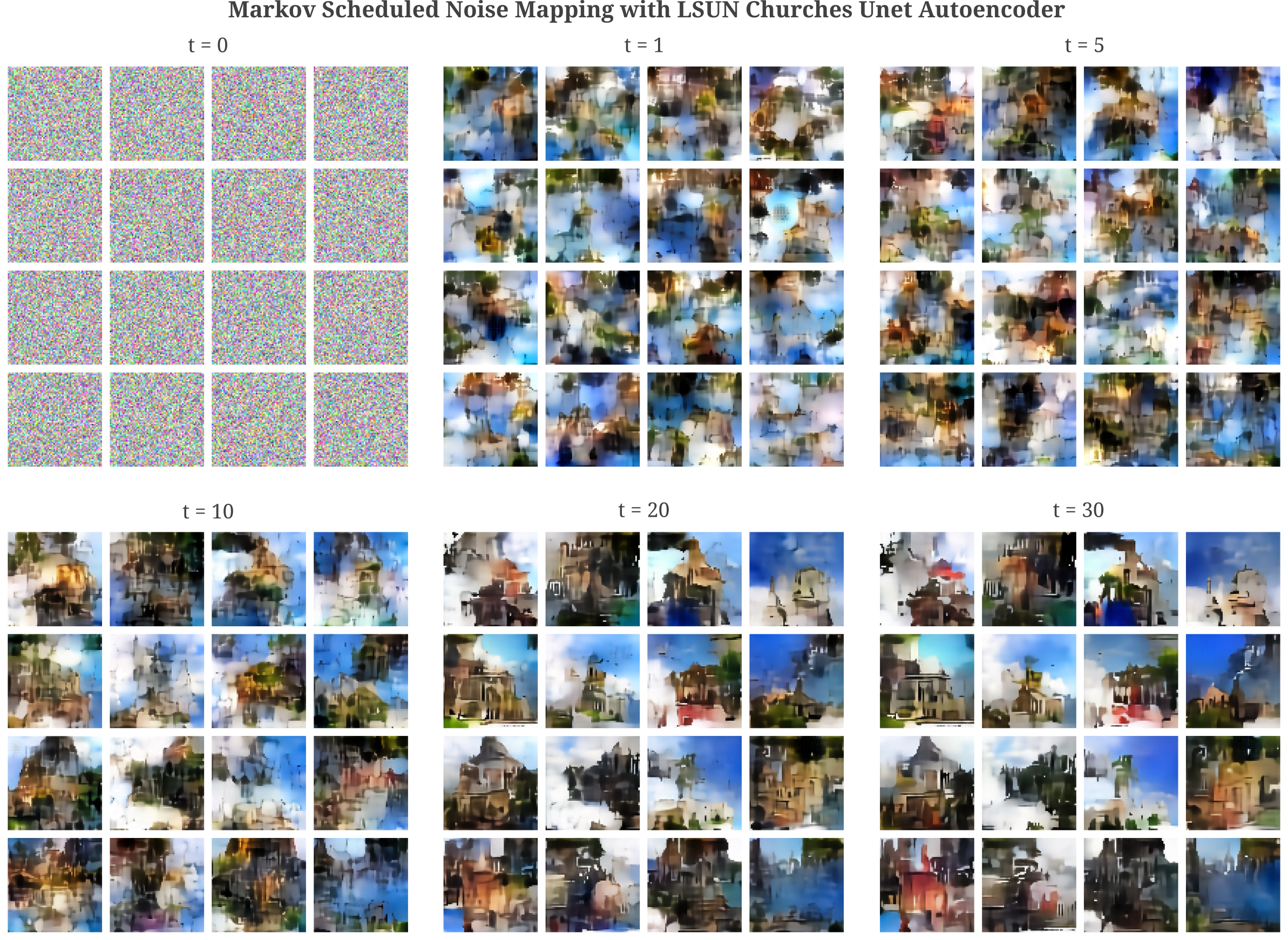
\[a_{n+1} = c * \mathcal D( \mathcal E(a)) + d * \mathcal N(a; \mu, \sigma)\]

Arguably the simplest schedule is a linear one in which $c = n / N$ and $d = 1 - (n/N)$. This works fairly well, and for 30 steps we have the following for a Unet trained on LSUN churches (note that each time point $t=n$ corresponds to the model’s denoised output rather than $a_n$ which denotes a denoised output plus a new noise).

And for the same model applied to generate images over 200 steps, we have

This method of continually de-noising an image is conceptually similar to the method by which a random walk is taken around a learned manifold, detailed in the last section on this page. Close observation of the images made above reveal very similar statistical characteristics to those generated using the random manifold self-map walk in the video below

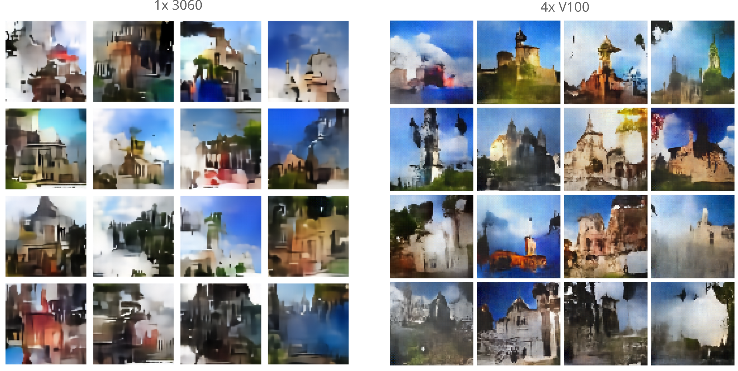
As is common for generative methods, applying larger models with more compute to the same dataset results in superior generative properties. This turns out to be true for autoencoders (Unet-style with no residuals) trained using MSE loss on the LSUN Churches dataset using the markov noise sampling method detailed above in the case where the model is larger and the compute power has increased a little more than tenfold. In the figure below, we compare the image generation results from 24 hours of training using 1x 3060 to the same timeframe but with 4x V100s, which for model training purposes results in a 10x-15x increase in throughput. Note the superior image detail, clarity, and realism in the images produced by the model trained using the larger compute cluster.

It is interesting to note that these statistical characteristics (for example, the dark maze-like lines and red surfaces on buildings that make a somewhat Banksy-style of generated image) are specific to the manifold learned. Observe that a similar model, Unet with a hidden MLP, as follows:

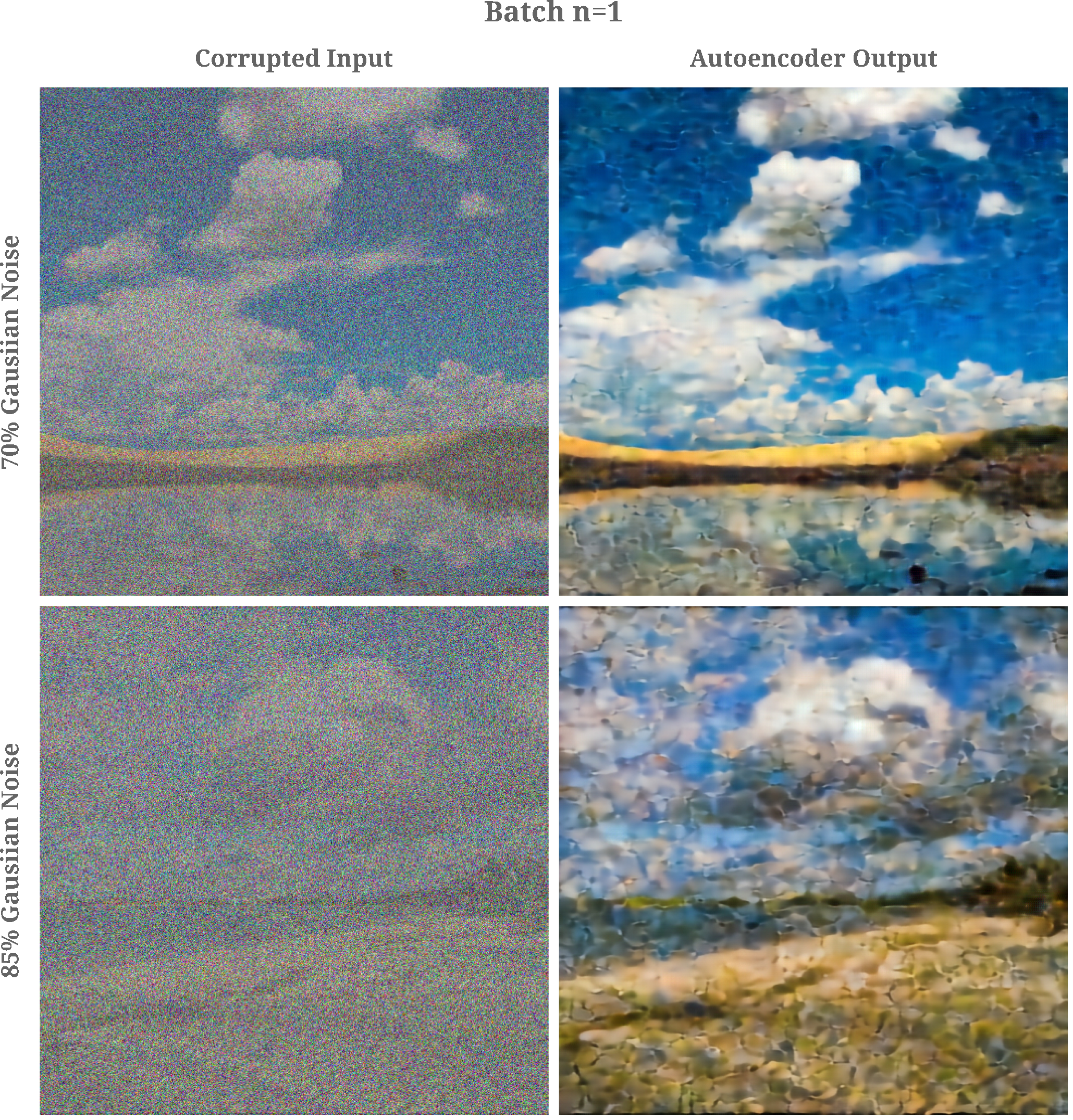
is capable of remarkable de-noising ability but tends to make oil painting-style characteristic changes during the denoising process.

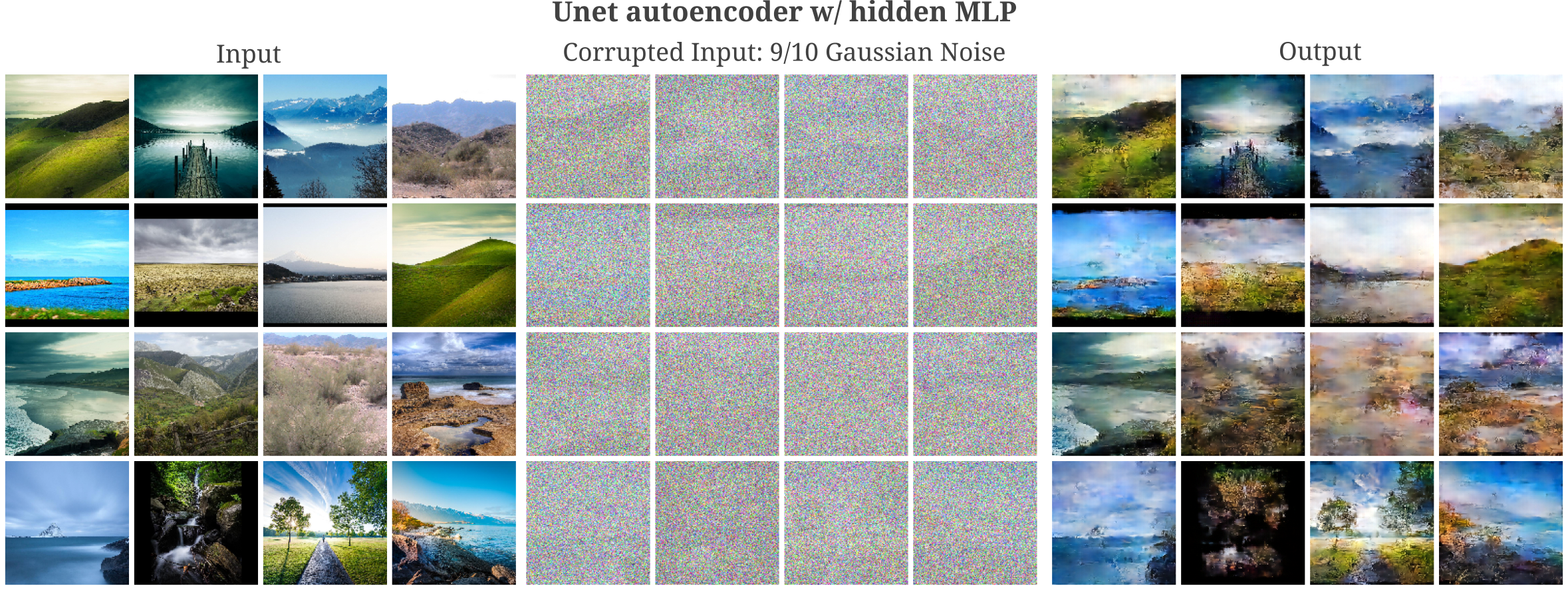
This suggests that the manifold learned when autoencoding images of landscapes (by this particular model) will also have oil painting-like characteristics. Indeed this appears to be the case, as when we use the diffusion-like markov sampling process to generate input images, we find that most have these same characteristics as well.

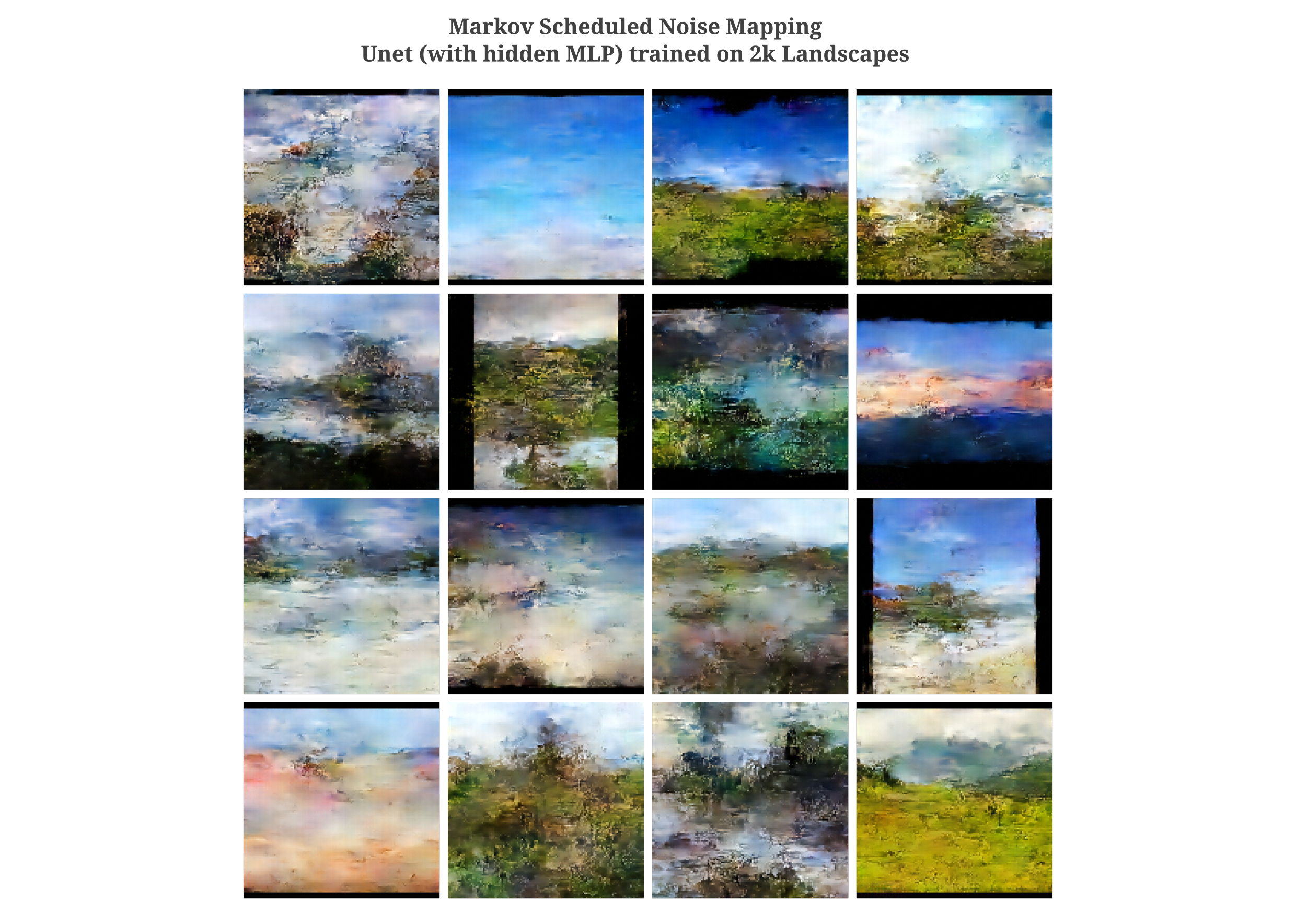
Increasing the number of iterations of the markov sampling process to 200, we have

For an increase in sampled image detail, one can increase the number of feature maps per convolutional layer in the Unet autoencoder architecture. With a model that has twice the layers per convolution as the standard Unet, we have the following:

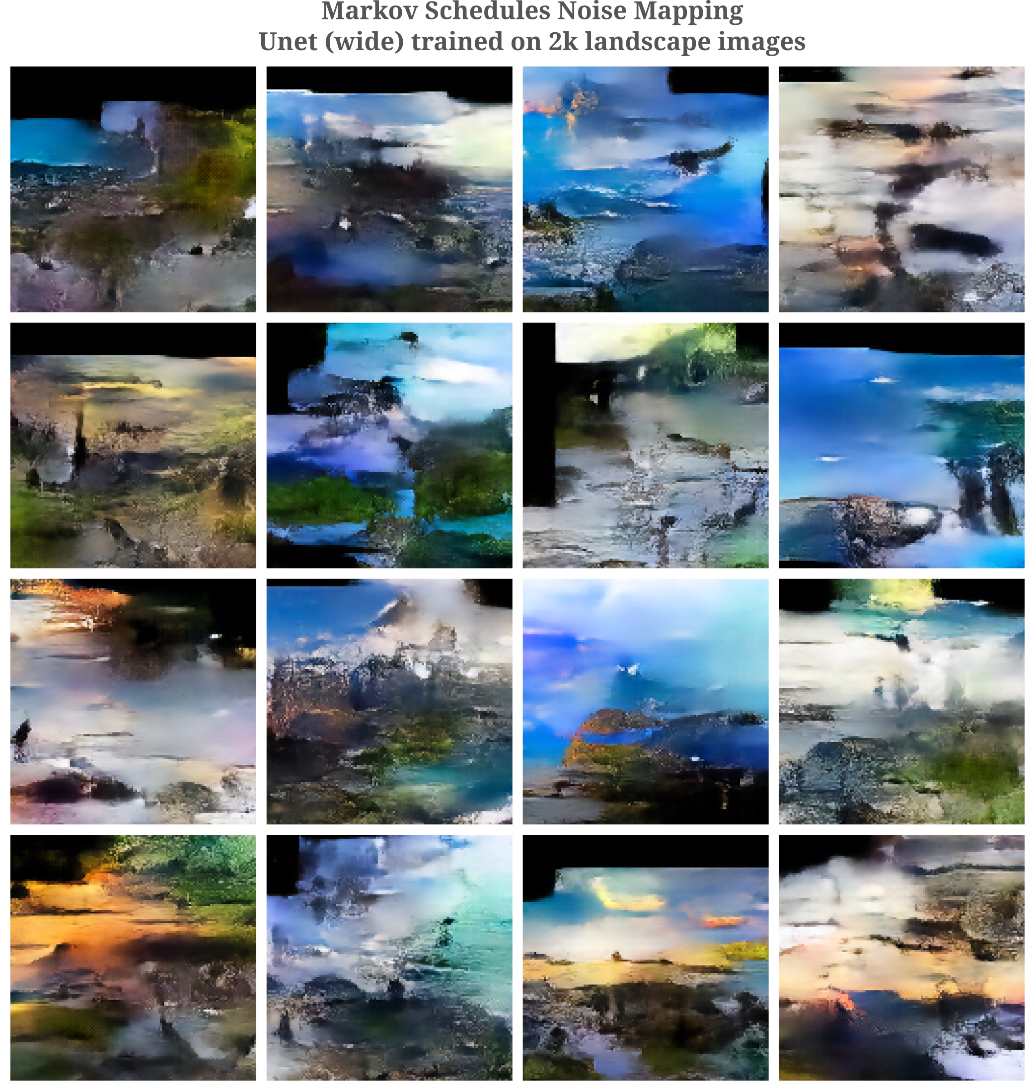
Although this model synthesizes images of greater detail and clarity that the narrower Unet, there are signs of greater global disorganization (black borders are often not straight lines, sky sometimes is generated under land).

One way to prevent this disorganization is to increase the number of convolutional layers present in the model (assuming fixed kernal dimension), and another is to employ at least one spatially unrestricted layer such as the fully connected layers above, or self-attention layers. We will investigate self-attention in later sections on this page, and for now will focus on increasing the number of convolutional layers.

To gain intuition for why this is, consider the following example: suppose one were to first take a single convolutional layer as the encoder and single up-convolution as the decoder. There would typically be no model parameters influencing both the pixels in the upper right and lower left of an input assuming that the convolutional kernal is significantly smaller that the input image dimension (as is usually the case). But then there is no guarantee that the model should be able to generate an image observing the ‘correct’ relationship between these two pixels as determined by the training dataset.

On the other hand, consider the extreme case in which many convolutions compose the input such that each image is mapped to a single latent space element, and subsequently many up-convolutions are performed to generate an output. There are necessarily model parameters that control the relationship of every pixel to every other pixel in this case.

Some experimentation justifies this intuition: when we add an extra layer to both encoder and decoder of the wide Unet, we obtain much more coherent images.

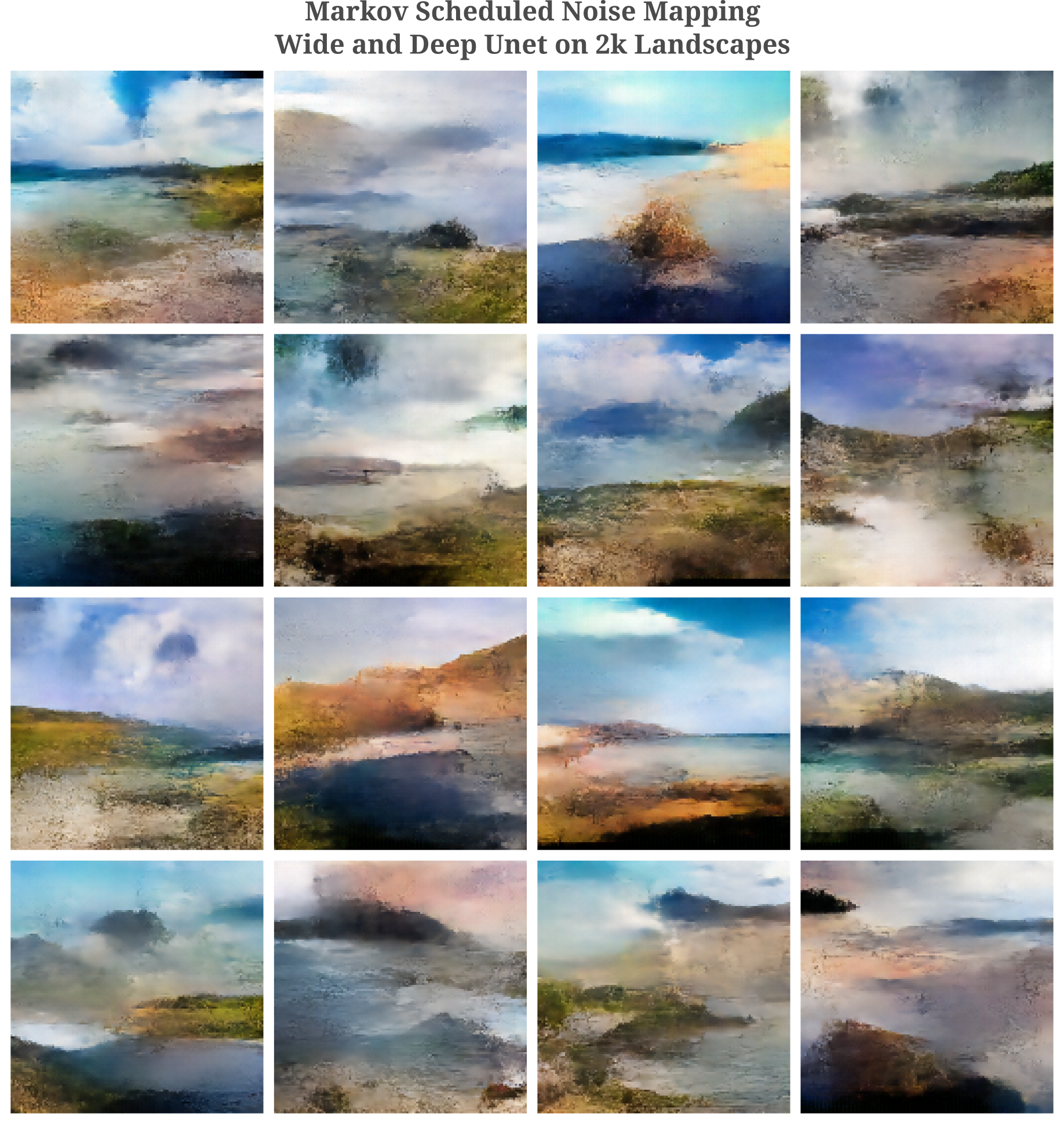
It is interesting to note that the extra width (more precisely doubling the number of feature maps per convolutional layer) reduces the number of painting-like artefacts present in the synthesized images after the diffusion-like generation process.

The Role of Batch Normalization in Denoising

Comparing the fully connected autoencoder to the Unet autoencoder, it is apparent that the latter is a more capable denoiser than the former. It is not particularly surprising that a larger and deeper model (the Unet) would be a better de-noiser than the former being that it can

\[y = \frac{x - \mathrm{E}(x_{m, n})}{\sqrt{\mathrm{Var}(x_{m, n}) + \epsilon}} * \gamma + \beta\]

where $m$ is the index of the layer output across all sequence items (ie convolutional filter outputs specified by height and width for Unet models) and $n$ is the index of the input among all in the batch.

Batch normalization odes play a role in the ability of Unet to denoise: removing batch normalizations from all convolutions in Unet results in autoencoder outputs that do not have noise per se, but are also statistically quite different than the original image. This does not affect the autoencoder’s ability to de-blur an input, however. Note that batch norm on this page is not switched to evaluation mode during image synthesis such that the model continues to take as arguments the mean and standard deviation statistics of the synthesized images.

On the other hand, it can be shown that this does not depend on the presence of a batch at all. We can retain Unet’s batch normalizations and simply train and evaluate a the model with batch sizes of 1 to remove the influence of multiple batch members on any given input. In effect, this removes index $n$ but not $m$ in the batch norm equation above. After training we see that this model is capable of around the same de-noising abilities that was observed with normal batch norm (ie with 8- or 16-size batches).

This provides evidence for the idea that the learning of $\gamma$ and $\beta$ only across a single image gives outputs that are statistically similar to the uncorrupted original input. One can think of batch normalization as enforcing general statistical principles on the synthesized images. For each layer (also called a feature map) of a convolution, batch normalization learns the appropriate mean and standard deviation across all samples $n$ in that batch and all spatial locations $m$ necessary for copying a batch of images. During the image synthesis process, batch normalization is capable of enforcing these learned statistics on the generated images.

It may be wondered whether batch normalization is necessary for accurate input representation in deep layers of the Unet autoencoder after training. The answer to this question is no, as with or without batch normalization the trained Unet output layer has equivalent representation ability of the input.

Representations in Unet generative models with Attention

It may be wondered why representation clarity (or lack thereof) would be significant. For tasks of classification, the importance of accurate input representation is unclear. One might assume that a poor representation accuracy in deep layers prevents overfitting, but as observed here the gradient descent process itself serves to prevent overfitting regardless of representational accuracy for classifiers. For generative models, however, there is a theoretical basis as to why imperfect deep representation is favorable.

To see why perfect input representation in the output may be detrimental to generative models, take a simple autoencoder designed to copy the input to the output. For a useful autoencoder we need the model $\theta$ to learn parameters that capture some important invariants in the data distribution $p(x)$ of interest. But with perfect input representation capability in the output the model may achieve arbitrarily low cost function value by learning to simply copy the input to output.

Next consider the case of a denoising autoencoder. This model is tasked with recoving the input $x$ drawn from the distribution $p(x)$ followed by a corruption process $C(x) = \tilde{x}$, minimizing the likelihood that the model output $ O(\tilde{x}, \theta) $ was not drawn from $p(x)$. Under some assumptions this is equivalent to minimizing the mean squared error

\[L = || O(\tilde{x}, \theta) - x ||_2^2\]

Now consider the effect of a perfect representation of the input $\tilde{x}$ in the output with respect to minimizing $L$. Then we have

\[L = || \tilde{x} - x ||_2^2\]

which is the MSE distance taken by the corruption process. Therefore the model is capable of inferring the corruption process without training.

These ideas have practical influence on the design of autoencoders when one attempts to add self-attention modules to the Unet backbone. Attention-augmented Unet architectures are typically used for Diffusion models in order to increase the expressivity of the model in question, and consist of Linear attention between high-dimensional (introduced by Katharopoulos and colleagues) and standard dot-product attention between lower-dimensional convolutional maps in parallel to residual connections.

The architecture we will use employs only linear attention, and may be visualized as follows:

But after training, it is apparent that this model is not very effective at de-noising

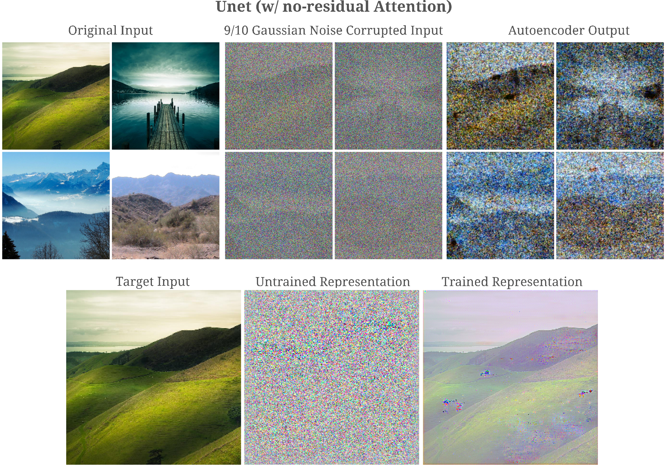
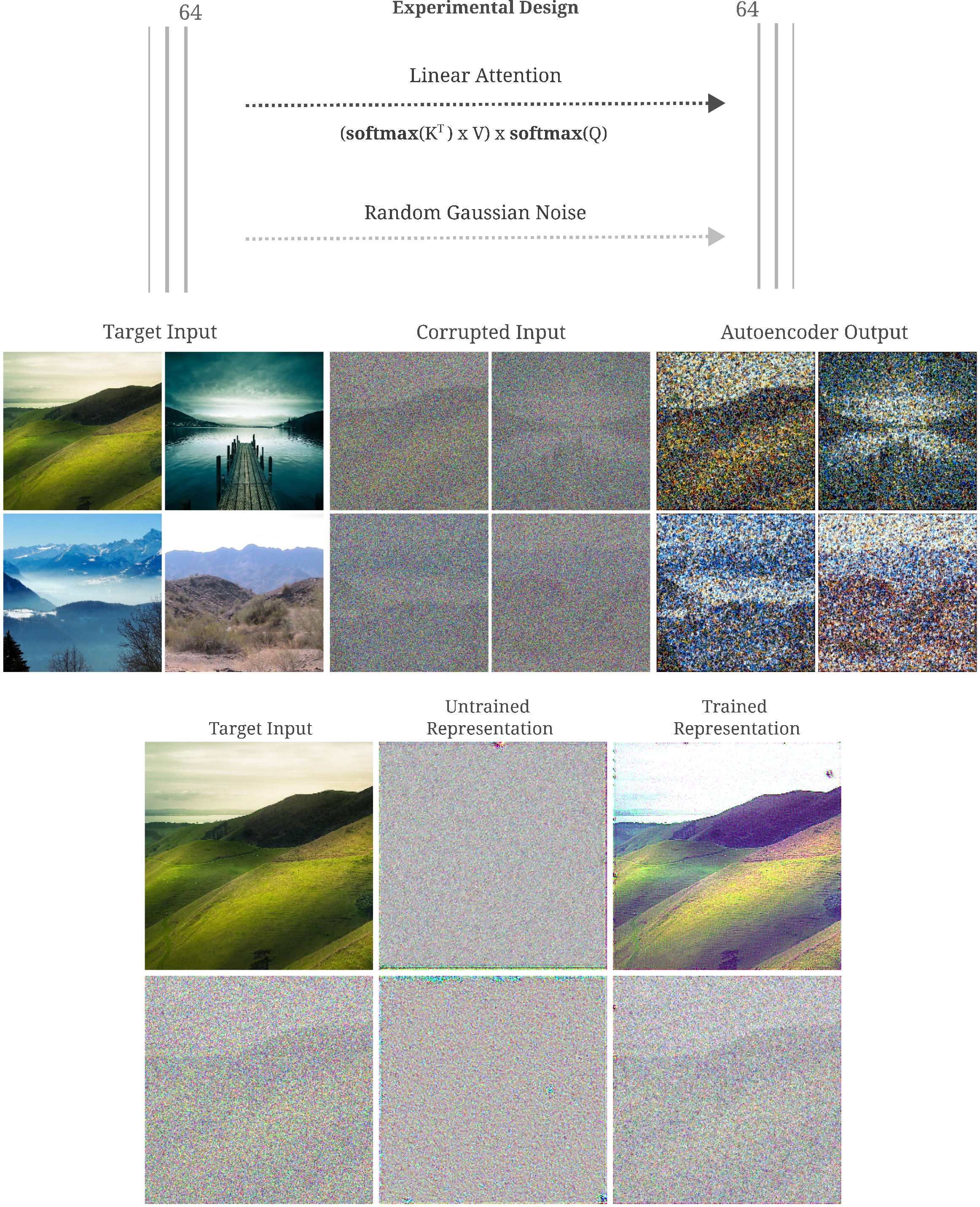
It may be wondered how much information is capable of passing though each linear attention transformation. If we restrict our model to just one linear attention transformation and input and output convolutions (each with 64 feature maps), we find that the model tends to learn to copy the input such that the model denoises the input poorly and is capable of near-perfect representation of its input, shown as follows:

Linear attention was introduced primarily to reduce the quadratic time and memory complexity inherent in the dot product operation in the normal attention module with linear-time complexity operations (aggregation and matrix multiplication). If we replace the linear attention module used above with the standard dot-product attention but limiting the input resolution to $32^2$ to prevent memory blow-up (while maintaining the input and output convolutions), we find that after training the autoencoder is capable of a less-accurate representation of the input than that which was obtained via linear attention.

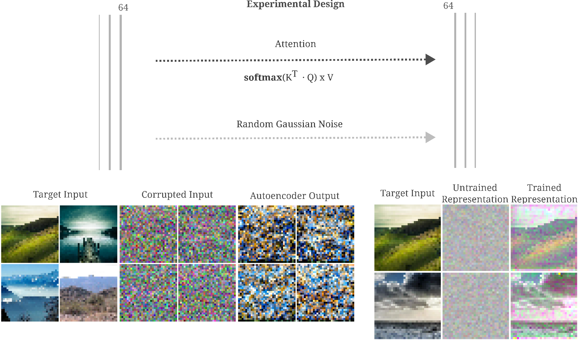
The input representation (of information present in the the output layer of our modified Unet) of the dot-product attention autoencoder in the last figure is surprisingly good given that dot-product attention is a strictly non-invertible operation. Indeed, if we remove input and output convolutions such that only dot-product attention transforms the input to the output, an effective autoencoder may be trained that is capable of good input representation (but does not denoise) as shown in the following figure.

This appears to be mostly due to conditioning: it is very difficult to generate an accurate representation across a dot-product attention transformation without a residual connection.

Conclusion

On this page we have seen that autoencoders learn to remove the noise introduced into their input representations via non-invertible transformations, and thus become effective denoising models without ever receiving explicit denoising training. The effect of this is that autoencoders may be used to generate images via a diffusion-like sampling process, and that one can observe the manifold learned by autoencoders is a similar way to that learned by generative adversarial networks.

Does this mean that we should all start using autoencoders to generate images and stop using diffusion models or GANs? Probably not, primarily because this approach relies on an implicitly trained ability rather than an explicitly trained one and secondarily because of the architectural limitations that autoencoders have.

What does it mean for a machine learning model to train explicitly for a task? The idea is that as we have seen on this page, autoencoders learn to denoise because the undercomplete linear transformations in each layer introduces noise into the model’s input representation before training, and this noise is removed as a result of MSE loss minimization on the output compared to input. The important thing to note there is that the process of denoising is itself never trained explicitly: one could imagine a model that minimizes autoencoder loss while not denoising at all, and indeed this is true for very small models.